ADCAIJ: Advances in Distributed Computing and Artificial Intelligence Journal
Regular Issue, Vol. 13 (2024), e32508
eISSN: 2255-2863
DOI: https://doi.org/10.14201/adcaij.32508
Evaluation of One-Class Techniques for Early Estrus Detection on Galician Intensive Dairy Cow Farm Based on Behavioral Data From Activity Collars
Álvaro Michelenaa, Esteban Jovea, Óscar Fontenla-Romerob and José-Luis Calvo-Rollea
a University of A Coruña, CTC, CITIC, Department of Industrial Engineering, Calle Mendizábal s/n, Ferrol, 15403, A Coruña, Spain
b University of A Coruña, LIDIA, CITIC, Faculty of Computer Science, Campus de Elviña, s/n, A Coruña
✉ alvaro.michelena@udc.es, esteban.jove@udc.es, oscar.fontenla@udc.es, jlcalvo@udc.es
ABSTRACT
Nowadays, precision livestock farming has revolutionized the livestock industry by providing it with devices and tools that significantly improve farm management. Among these technologies, smart collars have become a very common device due to their ability to register individual cow behavior in real time. These data provide the opportunity to identify behavioral patterns that can be analyzed to detect relevant conditions, such as estrus.
Against this backdrop, this research work evaluates and compares the effectiveness of six one-class techniques for estrus early detection in dairy cows in intensive farms based on data collected by a commercial smart collar. For this research, the behavior of 10 dairy cows from a cattle farm in Spain was monitored. Feature engineering techniques were applied to the data obtained by the collar, in order to add new variables and enhance the dataset.
Some techniques achieved F1-Score values exceeding 95 % in certain cows. However, considerable variability in the results was observed among different animals, highlighting the need to develop individualized models for each cow. In addition, the results suggest that incorporating a temporal context of the animal’s previous behavior is key to improving model performance. Specifically, it was found that when considering a period of 8 hours prior, the performance of the evaluated techniques was substantially improved.
KEYWORDS
precision livestock farming; cattle behaviour; intelligent monitoring collars; one-class techniques
1. Introduction
In recent decades, the global livestock sector has undergone a drastic transformation. One of the key factors affecting this industry is the growing demand for food, driven by demographic growth. The rise in demand implies the need to increase the production of meat products and by-products (Fukase and Martin, 2020). In this regard, there are numerous reports, and research works that have predicted and estimated significant increases in the demand for certain products such as milk (Ruviaro et al., 2020).
On the other hand, the number of livestock farms is currently decreasing considerably, especially in developed countries. The increase in production costs and the consequent reduction in profitability has led to the closure of many small and medium-sized farms (Rayas-Amor, 2005; Thornton, 2010).
In this context, livestock farms have undergone a significant transformation, characterized by an increase in their size and in the number of animals per farm. This intensive production model allows farmers to optimize resources, reducing production costs and, consequently, increasing their economic profitability. However, this centralized approach, although economically beneficial, poses significant challenges in efficient and ethical animal management (Neethirajan, 2020). The high concentration of animals in a confined space makes individualized monitoring difficult, which can delay early detection of disease, reproductive processes such as estrus, or issues related to animal welfare. In addition, the quest to maximize productivity can lead to unsustainable practices that are becoming increasingly relevant in the current context of climate crisis (Alonso et al., 2020; Niloofar et al., 2021).
To address these challenges, precision livestock farming (PLF) has emerged as an advanced alternative solution that leverages new technologies to improve livestock management. The main goal of PLF is to optimize production, ensure animal welfare and reduce environmental impact (Morrone et al., 2022). To achieve this, tools such as artificial intelligence (AI), the internet of things (IoT) and data analytics are applied, enabling real-time monitoring of animal health, nutrition and behavior (Garcia et al., 2020).
One of the most promising areas within PLF is the analysis of animal behavior, which allows for the early detection of diverse conditions, such as disease or gestation (Cocco et al., 2021). The capability to detect and interpret animal behavioral changes is crucial, as these can provide valuable information for early diagnostics, improved prognostics, and easier decision-making on livestock farms, maximizing both animal welfare and economic efficiency (Fogsgaard et al., 2015).
In terms of classifying, identifying and analyzing livestock behavior, various devices are currently in use, with smart monitoring collars being one of the most common. These devices include sensors such as accelerometers, gyroscopes and Inertial Measurement Units (IMU), which allow to record and differentiate between specific behaviors of the animal (Pratama et al., 2019). The ability to measure movements in different axes facilitates an accurate detection of activities such as grazing, ruminating, resting and so on (Michelena et al., 2024).
The data collected by these devices are increasingly combined with machine learning techniques and other advanced approaches for the detection of specific events in animal behavior. Among these events, heat detection is one of the most critical for farmers, as it directly affects the reproductive efficiency of beef and dairy farms (Michelena et al., 2024).
Estrus, or heat, is an essential part of the reproductive cycle of cows, as it indicates when they are ready to reproduce. Since the fertility window is short, accurate identification of estrus is key to maximizing production efficiency (Reith and Hoy, 2018). The estrous cycle in cows, which lasts 18 to 24 days, has an estrus phase that extends for only about 12 to 18 hours, during which cows exhibit typical behaviors such as increased physical activity, reduced feed intake and increased vocalization (Carvajal et al., 2020; Roelofs et al., 2005).
In addition, estrus causes physiological changes, such as hormonal variations in estrogen and progesterone levels, fluctuations in body temperature and an increase in vaginal secretion (Fesseha and Degu, 2020; Riaz et al., 2023). These indicators are fundamental to determine the best time for artificial insemination or mating, and to detect reproductive problems such as anestrus, a condition that affects fertility and, therefore, productivity in cattle.
Accurate and early estrus detection is essential to increase the success rate in gestation and, consequently, to improve the economic profitability of cattle farms (Gautam, 2023). Traditionally, heat detection was done by visual observation. However, with the reduction of estrus time and the increase in farm size, this method has proven to be inefficient, prompting the development of automated systems that employ sensors such as accelerometers in activity collars, pedometers or ear tags (Silper et al., 2015).
With the development of artificial intelligence, algorithms such as LSTM and CNN neural networks, among other machine learning methods, have been successfully implemented to analyze sensor data and detect estrus patterns (Ma et al., 2020; Thanh et al., 2018; Wang et al., 2020). Technologies such as computer vision, thermography, and temperature sensors or intravaginal devices have also been explored (Bruyere et al., 2012; Riaz et al., 2023).
Considering the importance of accurate heat detection, this paper analyzes and compares the performance of six one-class techniques for early heat detection using behavioral data obtained from an intelligent monitoring collar. The aim of this research is to develop an effective tool for early detection and identification of this reproductive behavior, in dairy cattle on intensive farms.
This paper is structured as follows: after the introduction, Section 2 presents a description of the smart collar that has been used, as well as details of the farm where the animals were monitored and of the collected dataset. Section 3 provides a brief definition of each of the six one-class techniques analyzed in this research, while Section 4 gives a detailed description of the experimental setup. The analysis of results is presented in Section 5, and finally, conclusions and future work are presented in Section 6.
2. Case study
This section describes both the main features of the smart collar used for monitoring cow behavior and the dataset that has been collected and used for the development of this research work.
2.1. Intelligent cattle monitoring collar
Currently, there are many enterprises that design and develop a wide variety of commercial devices for monitoring livestock behavior and other useful parameters. On the market, devices that incorporate different sensors, advanced algorithms, and communication protocols are available for the monitoring of animal-related data with high precision. They provide very valuable information for the management of livestock farms.
To carry out this research work, the Galician startup Innogando, a company specialized in the development of innovative devices and tools for livestock monitoring, has collaborated with the research team. In this regard, the device used for data collection was the RUMI Smart Collar, an intelligent collar developed by this startup specifically for monitoring cows' behavior. This device is shown in Figure 1.

Figure 1. RUMI Smart Collar
This device is equipped with GPS location technology and different high-precision sensors, such as accelerometers, designed to monitor the animal's daily activities accurately and continuously. For confidentiality reasons, we cannot provide further information about all the sensors included in the collar.
The RUMI Smart Collar not only allows to track the animal's specific location, but it is also capable of detecting and recording the key behaviors of these animals in real time. In this regard, the device applies algorithms based on artificial intelligence and data analysis to detect the following five behaviors: resting, ruminating, grazing, walking and playing, this last behavior corresponds to a more spontaneous and random behavior that is not clearly classified in any of the other ones. In addition, the device is also able to record the number of steps taken by the animal.
This device is designed to be placed on the left side of the cow's neck, at mid-height, by means of a heavy-duty interlocking nylon strap. This strap ensures the device is placed correctly, avoiding possible chafing of the animal's skin. To ensure the correct positioning of it, a small counterweight is placed on the lower part of the animal's neck using the same nylon strap with which the device is fixed. Both the system and the counterweight do not compromise the animal's welfare and allow total freedom of movement.
On the other hand, this collar is very robust and impact resistant. Both its design and manufacture allow it to withstand the demanding conditions of the livestock sector. The device has an IP67 encapsulated protection that guarantees correct functioning in the most adverse weather conditions, such as heavy rains or dusty environments. In addition, its ABS plastic housing provides additional protection against UV rays, enhancing the durability of the device under direct sunlight.
One of the most innovative features of the RUMI Smart Collar is its ability to self-charge by means of a small solar plate incorporated on its surface. This plate allows the device to recharge its batteries continuously, ensuring prolonged use without the need to replace or recharge the batteries manually. According to the manufacturer's specifications, in low sunlight conditions, the system is capable of continuing to operate for up to 8 months thanks to its high-capacity batteries and the device's low energy consumption.
For data transmission, the collar uses the LoRaWAN protocol. This protocol allows data to be sent over long distances with minimal power consumption, ensuring that information is collected and transmitted efficiently (Jabbar et al., 2022). The data generated by the device is sent from the collar to a gateway, which sends it to a centralized server through the Internet. Once stored, the data can be accessed by the farmer through a mobile application or from a computer, facilitating real-time monitoring and livestock management.
2.2. Dataset description
For this research work, an intensive dairy farm located in Outes village, in the southwestern province of A Coruña, Galicia, Spain, was selected. This farm has a total of 150 Holstein/Friesian cows, one of the most common breeds in the dairy industry due to its high milk production. Despite the high number of animals on this farm, for this research, and due to the complexity of the labeling process that will be discussed at the end of this section, a total of 10 non-pregnant cows of different ages, were selected for monitoring from March 7 to June 11, 2024 (95 days).
Each cow was monitored individually and continuously using the Rumi Smart Collar, previously described in Section 2.1. Specifically, the dataset includes the total minutes each cow spent on various activities (resting, ruminating, grazing, walking, and playing) during a given hour, as well as the number of steps taken in that hour. Since the cows were monitored separately, each collar contained a unique identifier (ID) that allowed the data associated with each animal to be differentiated and grouped.
Although the selected farm is an intensive farm, which means that the cows do not graze on pasture, the data recorded periods when some cows appeared to be grazing. This behavior is attributable to the fact that the cows consume feed or silage at ground level, an activity that the monitoring device may confuse with grazing behavior due to the similarity in cow movements and posture.
In addition to the previously mentioned variables, this labeled dataset also contains a binary variable indicating the behavioral pattern of the animal. This variable is 0 if the sample corresponds to a normal behavior pattern and 1 if the behavior pattern is linked to an abnormal behavior associated with estrus. Veterinarians, experts from the company Innogando and farm workers participated in the data labeling. For this purpose, visual observations of the livestock behavior were made several times a day, supported by cameras that enabled remote monitoring.
Given the complexity of labeling events at an hourly rate, the labeling process was developed as follows: when an anomalous behavior was observed in an animal, a waiting period was implemented to confirm if this behavior persisted. If so, all records between the first moment of detection and the return to typical behavior were labeled as anomalous.
Overall, the dataset contains a total of nine features:
•A timestamp, indicating the date and time to which the data corresponds.
•An ID variable containing the animal identification number to which the registered data are associated.
•Five numeric variables which contain the number of minutes the cow spent performing each of the five behaviors detected by the device in a given hour.
•A numeric variable containing the number of steps taken by the cow in a given hour.
•A binary label indicating whether the behavioral pattern identified in that hour corresponds to a typical or heat-related behavior.
Finally, it is very important to note that, as expected, the dataset is heavily unbalanced. A total of 22942 behavioral samples have been recorded, of which only 415 correspond to anomalous patterns, which represents 1.8 % of the dataset.
3. Application of one-class methods
In this research work, the performance of six different one-class techniques is evaluated and compared with the aim of assessing their performance for the identification of estrus in intensive-farming dairy cows. A brief definition of each of the applied techniques is provided in this section.
3.1. Principal component analysis
Principal component analysis (PCA) is a technique frequently used for dimensionality reduction in various fields, as well as for classification and regression tasks (Greenacre et al., 2022). Its main goal is to perform a linear transformation of the original dataset to a lower dimensional space, while preserving the most significant information. This transformation is based on the computation of the eigenvalues and eigenvectors of the covariance matrix. The eigenvectors reveal the directions in which the data show the greatest variability (Al-Qudah et al., 2023).
After projecting the data onto the linear subspace using the eigenvectors, the reconstruction error, defined as the distance between the original points and the projections of the original points onto the target subspace (D. M. J. Tax, 2001), is evaluated.
Figure 2 illustrates an example of how PCA is applied in a one-class scenario in ℝ2 using a principal component. In this case, the test instance (blue dot) is considered anomalous because it is farther away from the instances in the training set (red dots).
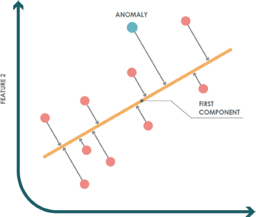
Figure 2. PCA example for anomaly detection
3.2. K-means
The K-means algorithm is an unsupervised technique widely used in various fields, such as machine learning, image processing and pattern detection among others (Annas and Wahab, 2023; Sinaga and Yang, 2020). Its main goal is to segment the dataset into groups or clusters composed of points with similar characteristics (Hu et al., 2023).
In a one-class approach, this algorithm is used to model the whole target set into several clusters. To determine whether a test instance is anomalous or not, the distance of that instance to the centroid of the nearest cluster is calculated.
Figure 3 shows an example in ℝ2, where the training set has been divided into three clusters. The gray dot represents a test instance that is considered anomalous, since the distance to its nearest centroid is greater than the maximum distance allowed within that cluster.
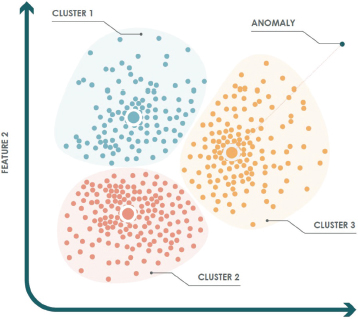
Figure 3. K-means example for anomaly detection
3.3. k-nearest neighbors
The k-nearest neighbors’ method, commonly known by its acronym KNN, is based on identifying samples that are close to each other, assuming that there is a relationship between them (Bansal et al., 2022). In this way, new data is classified as belonging to the target class if the distance to its nearest neighbor is less than a threshold previously determined during the training phase (Abu Alfeilat et al., 2019; Z. Zhang, 2016).
To estimate the local density, considering a dataset of given dimension, a hypersphere centered on a point belonging to the target class is constructed (Scott, 2015). The volume of such a hypersphere is expanded until it contains k =1 samples from the training set. In the specific case where k=1, a test data z is considered to belong to the target class if its local density is equal to or greater than that of its nearest neighbor within the training set.
In essence, in this method the classification process is reduced to comparing the distance between the test sample and its nearest neighbor, with the distance of the latter to its nearest neighbor. In this way, it is not necessary to explicitly calculate the density.
An example of the application of this technique for a class in ℝ2 with k=1 is illustrated in Figure 4. In this case, training instances are represented by blue dots, while a test sample is shown as an orange dot. This sample does not belong to the target class, since the distance to its nearest neighbor d1 is greater than the distance from that neighbor to its own nearest neighbor d2.
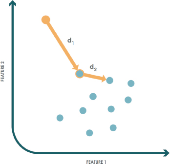
Figure 4. K-NN example for anomaly detection
3.4. Minimum spanning tree
The minimum spanning tree (MST) algorithm is used to construct a fully connected, undirected graph where the edges link pairs of instances from the original target set (Juszczak et al., 2009). This graph is generated under the assumption that two similar samples belonging to the target class should be close to each other (La Grassa et al., 2022). Considering the continuity within the target set, there should be a continuous transformation connecting these two samples. The MST algorithm connects points by tracing edges that minimize the distance between them, thus forming the graph.
Once the tree is constructed, the criterion to determine whether a new test sample X is anomalous is as follows: first, the point is projected onto its nearest edge Xp. If the distance between the point and its projection exceeds a predefined threshold, the sample is considered anomalous. Otherwise, it is classified as part of the target class (Juszczak et al., 2009). Figure 5 illustrates an example where an MST graph is applied to a two-dimensional dataset.
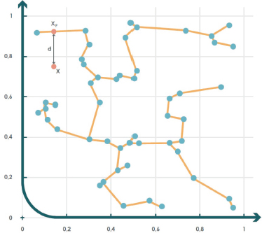
Figure 5. MST example for anomaly detection
3.5. Approximate convex hull
An intuitive approach to determine the geometric limits of a target set is by estimating the convex envelope that encloses all samples (Fernández-Francos et al., 2017). However, this procedure entails an exponential computational cost when working with high-dimensional datasets. Therefore, a new approach based on convex envelope computation is proposed in (Casale et al., 2011). This method consists of projecting the training set onto a random set of two-dimensional subspaces and then computing the convex envelope of the projected data. This approach, known as approximate convex hull (ACH), allows unexpected events to be detected when the projected input samples fall outside at least one of the n convex envelopes generated during the training phase.
Figure 6 shows an example in which a training set in ℝ3 (left graph) is projected onto two random subspaces to compute the corresponding convex envelopes (right graphs). Subsequently, a test instance (orange dot) is considered outside the target class if it lies outside at least one of the convex envelopes of the projections.
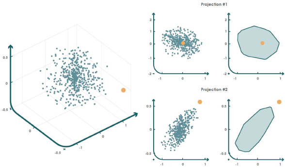
Figure 6. ACH example for anomaly detection
3.6. Non-convex boundary over projections
The non-convex boundary over projections (NCBoP) algorithm introduces an innovative approach by using nonconvex envelope calculations to represent the structure of the target dataset (Jove et al., 2021).
The NCBoP method constructs a nonconvex polygon for each 2D random projection, starting by selecting as the initial point the one with the lowest y coordinate among the projected points in the new 2D subspace. Then, the k closest points are identified and ordered according to the polar angle, retaining only the most distant point with respect to the initial one.
After calculating these first points, a stack structure is created to incorporate the third sample. Then, it is checked whether the next point in the list turns to the left (it is added to the stack) or to the right (the top point is removed). This cycle continues until the run is completed and returns to the starting point. Also, this process is repeated for each two-dimensional random projection.
Once the training stage is completed, the algorithm uses the following criterion to identify anomalies: if a new test point is outside at least one of the projected envelopes, it is considered anomalous. This concept is exemplified in Figure 7.
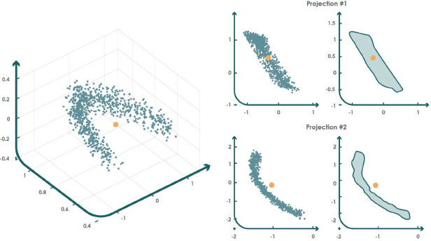
Figure 7. NCBoP example for anomaly detection
4. Experimental setup
This section describes the detailed steps followed to execute the proposal and the experiments carried out in this research work. For a better structure, the section is divided into several subsections.
4.1. Data preprocessing
Data preprocessing was initialized by splitting the data for each cow, which resulted in transforming the original dataset into 10 subsets (since, as mentioned, 10 cows were monitored), each corresponding to a specific animal. This dataset separation is due to the fact that in this research we have evaluated the performance of the one-class techniques described in Section 3 in individual cow models, since there can be significant differences between the behavior of one animal with respect to another, which can compromise the performance of these techniques in herd models where data of different animals are taken into account.
With the data segregated, the presence of missing hourly records in each of the 10 subsets was verified. The missing data were completed using the values of the previous hour for that cow, with the aim of maintaining temporal continuity and minimizing the loss of information.
4.2. Feature engineering: aggregation of information
The next step was the addition of new variables to the original dataset variables: resting, ruminating, walking, grazing, eating/playing and number of steps. This procedure, known as feature engineering, improves the quality of the models by providing additional and potentially more representative information (Zheng and Casari, 2018).
From the original variables, six new features were generated, corresponding to the sum of each activity and the number of steps over a previous hour. An example of this process using a three-hour period is shown in Figure 8.
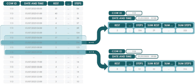
Figure 8. Example of new variable aggregation
This step is crucial, since estrus manifests itself as a change in behavior over several consecutive hours. Without the addition of these new variables, and as a consequence of the hourly frequency of the dataset, a model could detect any isolated anomalous behavior as estrus, without distinguishing it from real estrus. The new variables make it possible to collect behavior accumulated over n previous hours, which provides highly valuable information for the purposes of this research.
To evaluate the performance of the one-class techniques, six accumulation intervals were considered: 12, 8, 6, 4, 3 and 2 hours. This resulted in multiple data configurations, each representing a different temporal level of analysis.
In addition, an extra numeric feature was added to represent the time slot of each record. Cows, like other animals, present variations in their behavior throughout the day, influenced by circadian rhythms (Reith and Hoy, 2018; Roelofs et al., 2010). In addition, in an intensive system, the cows' hourly behavior tends to be more marked and predictable due to the strict routine in feeding and management. When detecting estrus, considering the time of day is important, as estrus tends to occur mainly during the night or early morning hours, which provides additional information to the detection of estrus episodes (Reith and Hoy, 2018).
At the end of the process, each subset of data has a total of 13 variables and the binary label indicating normal behavior or estrus. In addition, since new features were created based on six different time intervals and individual subsets were generated for each cow, the preprocessing resulted in 60 independent datasets (6 configurations for each of the 10 cows).
4.3. Configuration of the one-class methods
For each of the 60 datasets generated by applying the procedure explained above, each of the one-class methods described in Section 3 was trained and evaluated.
To optimize the performance of each of the implemented one-class methods, an accurate tuning of their hyperparameters was performed. For each technique, different configurations of parameters were explored to identify the optimal values. The configured hyperparameters and the values used for each technique are listed below.
•Principal component analysis
∘Number of components: 1:1:12 components.
∘Dataset outlier fraction considered during the training phase: 0:0.05:0.15.
•K-means
∘Number of clusters: 1:1:30 clusters.
∘Dataset outlier fraction considered during the training phase: 0:0.05:0.15.
•k-nearest neighbors
∘Number of neighbors: 5, 10, 20, 25, 30 and sqrt(number of training samples) neighbors.
∘Dataset outlier fraction considered during the training phase: 0:0.05:0.15.
•Minimum spanning tree
∘Dataset outlier fraction considered during the training phase: 0:0.05:0.15.
•Approximate convex hull
∘Number of 2D projections: 10, 50, 100, 200, 400, 600, 800 and 1000 projections.
∘Lambda: this parameter allows to contract or expand the vertexes of the convex hull. Values less than 1 are used to contract while values greater than 1 are used to expand. The values tested in this research work were 0.8:0.2:1.4.
∘Data center: Centroid.
•Non-convex boundary over projections
∘Number of 2D projections: 10, 50, 100, 200, 400, 600, 800 and 1000 projections.
∘Lambda: 0.8:0.2:1.4.
∘Data center: Centroid.
On the other hand, it is also important to note that each different model configuration has been evaluated for three different dataset normalization processes:
•Normalization in the range 0-1 (“Norm”).
•Normalization z-score, with mean 0 and standard deviation 1 [43] (“ZScore”).
•Non-normalized data (“NoNorm”).
4.4. Training, validation and evaluation of classifiers
For the training process, a cross-validation process with a k-fold of 5 was implemented and repeated two times in order to provide robust results that accurately reflect the performance of the selected techniques and methodology in the early detection of estrus in dairy cows (X. Zhang and Liu, 2023). This procedure was carried out for each of the different configurations of each technique as well as for each of the subsets generated from the original dataset.
The whole training and experimental process was carried out in Matlab R2023b using the toolbox dd_tools (D. Tax, 2018). Figure 9 provides a schematic representation of the workflow followed during the model training and validation process.

Figure 9. Training model and training samples
As illustrated in Figure 9, it is essential to note that since these are one-class techniques, anomalies are not included in the training of the models. Thus, the records associated with estrus behavior are only used for the validation process. This feature is crucial for the correct application of anomaly detection methods, where the main goal is to identify atypical and unknown behaviors during the training phase.
On the other hand, it must be taken into account that the dataset presents a significant imbalance between classes, so the selection of an appropriate metric is fundamental to compare and validate the different models that have been generated. In this case, the F1-Score was used, which is the harmonic mean between precision and sensitivity, whose mathematical expression is defined in Equation 1.
Considering that Precision is defined by Equation 2 and Sensitivity by Equation 3, the f1 score can also be defined as a ratio of true positives to false positives and false negatives, as shown in Equation 4. In these three equations FP indicates False Positives, FN corresponds to False Negatives and TP indicates True Positives.
The F1-Score is particularly valuable in anomaly detection tasks with unbalanced data, as it trades-off the need to capture a high number of anomalies (high sensitivity) and ensures that the assigned anomaly labels are accurate (high precision). The F1-Score metric is therefore effective for evaluating anomaly detection models. It prevents the model from being biased towards the majority class, penalizing performance if the model fails to detect anomalies (Raschka, 2014).
Although the F1-Score is usually represented in values between 0-1, in Section 5 the scores are given in percentage to simplify the interpretation of the results. A value of 100 \ % suggests that the model has classified all estrus samples correctly, with no false positive or false negative.
In addition, due to the cross-validation process, the standard deviation of the F1-Score is estimated. This measurement provides information on the variability in model performance over the different cross-validation iterations. A low standard deviation reflects that the model is robust and produces similar results across the different training and test folds. Conversely, a high standard deviation may suggest that the model performance is highly dependent on the subset of data used for training.
Measuring the standard deviation also allows to detect overfitting issues. If exceptionally high performance is observed for some folds and low for others, it could be indicative that the model is over-fitting in certain data subsets.
Since the F1-Score metric is measured in percentage, the standard deviation is also evaluated in the same way, providing a percentage measure of the variability between the different models evaluated during cross-validation.
5. Results analysis
In this section, the results obtained throughout the development of the research work described in this article are shown and analyzed. As previously mentioned, numerous configurations have been evaluated in this study, including hyperparameter settings for each of the implemented techniques, different data normalization methods, as well as different time intervals considered for the generation of new variables.
Each of the model configurations, together with the different normalization methods, has been applied and evaluated for each of the 60 datasets generated. This approach has provided a considerable volume of results, due to the diversity of models and configurations analyzed. Therefore, in order to simplify the interpretation of these results, this section shows only those that have achieved the highest F1-Score percentages, allowing us to identify the most effective settings.
This section has a twofold aim. On the one hand, we seek to determine which are the best one-class techniques, as well as the optimal configurations for early estrus detection in dairy cattle in intensive farms. On the other hand, the performance of these techniques is analyzed as a function of the time interval considered to generate the new variables. This will allow for a better understanding of the factors that contribute to the successful detection of estrus behaviors and the development of an animal health monitoring tool that responds early and accurately to these behaviors.
5.1. Analysis of one-class techniques
A detailed analysis of each of the implemented one-class techniques is discussed in detail below. For each technique, the configurations that performed best for each of the generated subsets of data are presented. The purpose of this section is not only to evaluate the overall performance of each technique for each animal, but also to identify the configurations that have obtained the best results.
5.1.1. Principal component analysis results
The results obtained by applying PCA on each data subset are presented in Table 1, which gives the configurations with which the best results were obtained among all those evaluated.
Table 1. PCA results
Cow ID |
Hours considered |
Normalization |
Number of components |
Outlier fraction |
F1-Score (%) |
Standard deviation (%) |
4 |
2 |
Norm |
8 |
0.05 |
74.55 |
3.83 |
4 |
3 |
Zscore |
9 |
0.05 |
79.72 |
1.99 |
4 |
4 |
Zscore |
9 |
0.05 |
81.38 |
3.77 |
4 |
6 |
Zscore |
9 |
0.05 |
83.24 |
2.71 |
4 |
8 |
Zscore |
6 |
0.05 |
84.82 |
2.98 |
4 |
12 |
Norm |
12 |
0 |
87.85 |
1.20 |
57 |
2 |
Zscore |
4 |
0.05 |
65.81 |
6.71 |
57 |
3 |
Zscore |
7 |
0.05 |
65.44 |
3.84 |
57 |
4 |
Zscore |
6 |
0.05 |
67.51 |
5.76 |
57 |
6 |
Norm |
9 |
0.05 |
68.29 |
5.07 |
57 |
8 |
Norm |
4 |
0.05 |
68.64 |
4.23 |
57 |
12 |
Norm |
4 |
0.05 |
72.86 |
4.22 |
58 |
2 |
Zscore |
3 |
0.05 |
83.75 |
3.92 |
58 |
3 |
Zscore |
8 |
0.05 |
82.99 |
3.12 |
58 |
4 |
Zscore |
8 |
0.05 |
84.59 |
2.89 |
58 |
6 |
NoNorm |
2 |
0 |
89.55 |
0.27 |
58 |
8 |
NoNorm |
2 |
0 |
89.76 |
0.25 |
58 |
12 |
Norm |
11 |
0 |
89.79 |
0.11 |
242 |
2 |
Zscore |
4 |
0.05 |
67.83 |
4.54 |
242 |
3 |
Zscore |
3 |
0.05 |
71.96 |
2.94 |
242 |
4 |
Zscore |
5 |
0.05 |
74.19 |
3.30 |
242 |
6 |
Zscore |
4 |
0.05 |
80.71 |
2.71 |
242 |
8 |
Zscore |
5 |
0.05 |
81.48 |
4.95 |
242 |
12 |
Zscore |
4 |
0.05 |
82.71 |
2.93 |
418 |
2 |
Zscore |
9 |
0.05 |
59.83 |
3.31 |
418 |
3 |
Zscore |
8 |
0.05 |
62.65 |
4.60 |
418 |
4 |
Zscore |
4 |
0.05 |
66.55 |
3.76 |
418 |
6 |
Norm |
1 |
0.05 |
67.47 |
3.18 |
418 |
8 |
Norm |
4 |
0.05 |
70.77 |
3.06 |
418 |
12 |
Norm |
4 |
0.05 |
73.42 |
4.47 |
659 |
2 |
Norm |
6 |
0.05 |
63.90 |
4.62 |
659 |
3 |
Zscore |
4 |
0.05 |
64.65 |
4.81 |
659 |
4 |
Zscore |
8 |
0.05 |
66.21 |
4.86 |
659 |
6 |
Zscore |
9 |
0.05 |
70.02 |
4.52 |
659 |
8 |
Zscore |
9 |
0.05 |
71.75 |
5.53 |
659 |
12 |
Zscore |
9 |
0.05 |
75.35 |
2.87 |
702 |
2 |
Zscore |
8 |
0.05 |
79.53 |
2.58 |
702 |
3 |
NoNorm |
1 |
0.05 |
81.67 |
2.82 |
702 |
4 |
Norm |
9 |
0.05 |
84.07 |
3.39 |
702 |
6 |
Norm |
12 |
0 |
89.15 |
0.76 |
702 |
8 |
Zscore |
12 |
0 |
92.93 |
1.22 |
702 |
12 |
Zscore |
12 |
0 |
91.91 |
0.28 |
870 |
2 |
Zscore |
4 |
0.05 |
60.71 |
2.45 |
870 |
3 |
Zscore |
5 |
0.05 |
63.61 |
4.24 |
870 |
4 |
Zscore |
5 |
0.05 |
67.76 |
2.75 |
870 |
6 |
Zscore |
5 |
0.05 |
69.64 |
2.58 |
870 |
8 |
Zscore |
5 |
0.05 |
71.86 |
2.07 |
870 |
12 |
Zscore |
9 |
0.05 |
72.84 |
0.94 |
874 |
2 |
NoNorm |
1 |
0.05 |
46.93 |
2.49 |
874 |
3 |
NoNorm |
2 |
0 |
49.94 |
2.39 |
874 |
4 |
NoNorm |
2 |
0 |
56.74 |
1.46 |
874 |
6 |
Norm |
10 |
0.05 |
61.30 |
7.39 |
874 |
8 |
Norm |
4 |
0.05 |
65.34 |
4.32 |
874 |
12 |
Zscore |
1 |
0.05 |
68.57 |
5.23 |
997 |
2 |
Norm |
3 |
0.05 |
68.74 |
4.05 |
997 |
3 |
Zscore |
5 |
0.05 |
71.81 |
3.06 |
997 |
4 |
Norm |
4 |
0.05 |
75.17 |
2.63 |
997 |
6 |
Zscore |
2 |
0.05 |
74.59 |
3.32 |
997 |
8 |
Zscore |
3 |
0.05 |
75.41 |
3.25 |
997 |
12 |
Zscore |
3 |
0.05 |
78.91 |
2.46 |
From the analysis of the results shown in Table 1, the following conclusions can be drawn:
•Regarding the PCA hyperparameters, the most frequent values for the number of components are 4 and 9, with an outlier fraction of 0.05. In terms of normalization, the Z-score method proved to be the most efficient in most cases, indicating that PCA generally requires a moderate number of components and prior normalization to optimize its performance.
•When looking at the performance as a function of F1 Score for all animals and different hour intervals, it is found that it varies between 46.9 % and 92.9 %, indicating a high variability among the different datasets.
•There is high variability in performance for each cow, suggesting significant differences in individual behavior patterns. In addition, longer data windows tend to improve model performance, indicating the need for more temporal context to obtain accurate results. It was also observed that when previous hours were considered, the standard deviation between models was reduced, making the models more stable and robust. In this regard, Figure 10 clearly illustrates these differences between animals and time configurations.
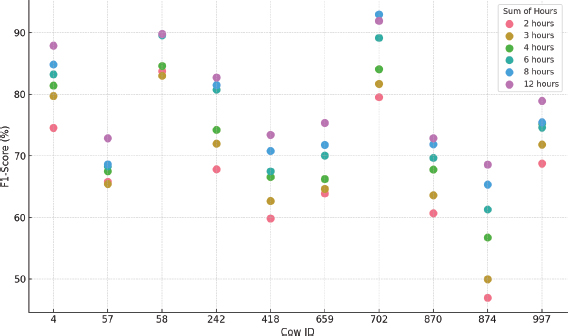
Figure 10. PCA F1-Score results for each cow and hours considered
5.1.2. K-means results
Table 2 collects the results of the K-means method applied to each data subset, showing the best performing configuration.
Table 2. K-means results
Cow ID |
Hours considered |
Normalization |
Number of clusters |
Outlier fraction |
F1-Score (%) |
Standard deviation (%) |
4 |
2 |
NoNorm |
1 |
0.05 |
75.67 |
3.85 |
4 |
3 |
NoNorm |
6 |
0.05 |
80.40 |
3.42 |
4 |
4 |
NoNorm |
2 |
0.05 |
82.67 |
3.29 |
4 |
6 |
NoNorm |
19 |
0 |
87.38 |
1.01 |
4 |
8 |
NoNorm |
17 |
0 |
92.80 |
0.38 |
4 |
12 |
NoNorm |
6 |
0 |
96.36 |
0.25 |
57 |
2 |
NoNorm |
1 |
0.05 |
66.23 |
5.59 |
57 |
3 |
NoNorm |
1 |
0.05 |
70.12 |
4.07 |
57 |
4 |
NoNorm |
1 |
0.05 |
70.31 |
5.63 |
57 |
6 |
NoNorm |
4 |
0.05 |
72.56 |
6.03 |
57 |
8 |
NoNorm |
1 |
0.05 |
75.17 |
3.11 |
57 |
12 |
NoNorm |
1 |
0.05 |
78.73 |
2.77 |
58 |
2 |
NoNorm |
2 |
0.05 |
82.85 |
3.03 |
58 |
3 |
NoNorm |
29 |
0 |
84.75 |
1.74 |
58 |
4 |
NoNorm |
25 |
0 |
90.49 |
3.46 |
58 |
6 |
NoNorm |
29 |
0 |
93.43 |
0.90 |
58 |
8 |
NoNorm |
25 |
0 |
93.48 |
0.31 |
58 |
12 |
NoNorm |
14 |
0 |
94.10 |
0.40 |
242 |
2 |
NoNorm |
1 |
0.05 |
73.48 |
3.47 |
242 |
3 |
NoNorm |
2 |
0.05 |
75.40 |
2.65 |
242 |
4 |
NoNorm |
24 |
0 |
79.17 |
0.87 |
242 |
6 |
NoNorm |
28 |
0 |
85.41 |
2.05 |
242 |
8 |
NoNorm |
30 |
0 |
85.37 |
2.10 |
242 |
12 |
NoNorm |
1 |
0.05 |
83.66 |
2.52 |
418 |
2 |
NoNorm |
1 |
0.05 |
66.98 |
4.41 |
418 |
3 |
NoNorm |
1 |
0.05 |
68.16 |
3.35 |
418 |
4 |
NoNorm |
1 |
0.05 |
71.93 |
4.18 |
418 |
6 |
NoNorm |
1 |
0.05 |
73.53 |
3.77 |
418 |
8 |
NoNorm |
1 |
0.05 |
74.30 |
4.51 |
418 |
12 |
NoNorm |
1 |
0.05 |
77.38 |
3.53 |
659 |
2 |
NoNorm |
3 |
0.05 |
68.82 |
4.56 |
659 |
3 |
NoNorm |
1 |
0.05 |
69.50 |
4.10 |
659 |
4 |
NoNorm |
14 |
0 |
77.31 |
1.11 |
659 |
6 |
NoNorm |
17 |
0 |
80.21 |
0.81 |
659 |
8 |
NoNorm |
9 |
0 |
86.31 |
0.57 |
659 |
12 |
NoNorm |
9 |
0 |
87.21 |
0.83 |
702 |
2 |
NoNorm |
26 |
0 |
81.09 |
2.80 |
702 |
3 |
NoNorm |
9 |
0 |
87.46 |
2.19 |
702 |
4 |
NoNorm |
21 |
0 |
91.22 |
3.15 |
702 |
6 |
NoNorm |
1 |
0 |
95.54 |
0.03 |
702 |
8 |
NoNorm |
1 |
0 |
95.84 |
0.14 |
702 |
12 |
NoNorm |
30 |
0 |
93.36 |
2.43 |
870 |
2 |
NoNorm |
1 |
0.05 |
69.11 |
2.09 |
870 |
3 |
NoNorm |
1 |
0.05 |
71.60 |
2.02 |
870 |
4 |
NoNorm |
1 |
0.05 |
73.76 |
1.29 |
870 |
6 |
NoNorm |
1 |
0.05 |
77.23 |
1.64 |
870 |
8 |
NoNorm |
27 |
0.05 |
78.26 |
1.34 |
870 |
12 |
NoNorm |
1 |
0.05 |
77.94 |
1.56 |
874 |
2 |
NoNorm |
1 |
0.05 |
58.38 |
5.26 |
874 |
3 |
NoNorm |
2 |
0.05 |
60.06 |
3.44 |
874 |
4 |
NoNorm |
2 |
0 |
65.51 |
0.65 |
874 |
6 |
NoNorm |
29 |
0 |
70.02 |
4.21 |
874 |
8 |
NoNorm |
3 |
0 |
74.74 |
1.22 |
874 |
12 |
NoNorm |
26 |
0 |
77.83 |
0.50 |
997 |
2 |
NoNorm |
1 |
0.05 |
71.84 |
3.39 |
997 |
3 |
NoNorm |
2 |
0.05 |
76.22 |
6.30 |
997 |
4 |
NoNorm |
29 |
0 |
77.93 |
1.55 |
997 |
6 |
NoNorm |
1 |
0 |
83.75 |
0.55 |
997 |
8 |
NoNorm |
3 |
0 |
84.26 |
0.12 |
997 |
12 |
NoNorm |
10 |
0.05 |
81.73 |
2.37 |
From Table 2, the following conclusions are highlighted:
•Regarding the hyperparameters of this technique, it was observed that the most common configuration involves the use of a single cluster, with a fraction of outliers varying between 0 and 0.05 depending on the dataset analyzed. The K-means method showed better performance without applying normalization.
•As with the PCA technique the F1 Score, which varies between 58.4 % and 96.4 % for all animals and different hour intervals, indicates high variability between datasets.
•Also, similar to PCA, there is high variability in performance per cow, suggesting significant differences in behavioral patterns. Longer data windows also improve model performance and reduce standard deviation. Figure 11 visually shows these differences between animals and time configurations when applying K-means.
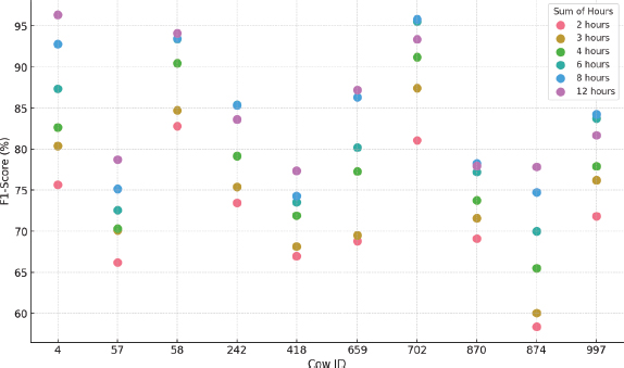
Figure 11. K-means F1-Score results by cow and hours considered
5.1.3. K-nearest neighbors results
The KNN results obtained in each data subset are presented in Table 3. Analyzing this table the following conclusions can be obtained:
•The number of neighbors varies significantly between the datasets, so no specific conclusions can be drawn in this regard. As in K-means, the fraction of outliers varies between 0 and 0.05, and the best results are generally obtained without normalization, except in two configurations that improved with z-score normalization.
•Similar to previous techniques, the F1 Score varies considerably, ranging from 57.7 % to 96.4 % depending on the animal and hour interval. Longer data windows improve performance and reduce the standard deviation. Figure 12 illustrates the differences between animals and time settings when applying this method.
Table 3. KNN results
Cow ID |
Hours considered |
Normalization |
Number of neighbors |
Outlier fraction |
F1-Score (%) |
Standard deviation (%) |
4 |
2 |
NoNorm |
20 |
0.05 |
76.40 |
3.81 |
4 |
3 |
NoNorm |
5 |
0.05 |
80.39 |
3.34 |
4 |
4 |
NoNorm |
20 |
0.05 |
83.21 |
4.24 |
4 |
6 |
NoNorm |
30 |
0 |
86.35 |
1.60 |
4 |
8 |
NoNorm |
5 |
0 |
92.32 |
0.36 |
4 |
12 |
NoNorm |
sqrt(nº samples) |
0 |
96.36 |
0.25 |
57 |
2 |
NoNorm |
5 |
0.05 |
67.25 |
5.37 |
57 |
3 |
NoNorm |
10 |
0.05 |
70.73 |
3.61 |
57 |
4 |
NoNorm |
10 |
0.05 |
70.38 |
5.42 |
57 |
6 |
NoNorm |
10 |
0.05 |
73.38 |
4.90 |
57 |
8 |
NoNorm |
10 |
0.05 |
75.65 |
5.50 |
57 |
12 |
NoNorm |
0 |
0.05 |
79.09 |
3.28 |
58 |
2 |
NoNorm |
30 |
0.05 |
82.85 |
3.04 |
58 |
3 |
NoNorm |
20 |
0.05 |
83.84 |
3.06 |
58 |
4 |
NoNorm |
sqrt(nº samples) |
0 |
87.37 |
2.45 |
58 |
6 |
NoNorm |
30 |
0 |
93.26 |
0.04 |
58 |
8 |
NoNorm |
20 |
0 |
93.27 |
0.04 |
58 |
12 |
NoNorm |
10 |
0 |
93.88 |
0.15 |
242 |
2 |
NoNorm |
5 |
0.05 |
74.24 |
4.85 |
242 |
3 |
NoNorm |
30 |
0.05 |
76.43 |
4.73 |
242 |
4 |
NoNorm |
10 |
0.05 |
77.58 |
2.33 |
242 |
6 |
Zscore |
10 |
0.05 |
80.95 |
2.54 |
242 |
8 |
Zscore |
10 |
0.05 |
81.97 |
2.85 |
242 |
12 |
NoNorm |
10 |
0.05 |
83.73 |
3.65 |
418 |
2 |
NoNorm |
5 |
0.05 |
69.08 |
3.86 |
418 |
3 |
NoNorm |
5 |
0.05 |
70.05 |
2.67 |
418 |
4 |
NoNorm |
30 |
0.05 |
72.07 |
4.76 |
418 |
6 |
NoNorm |
30 |
0.05 |
72.82 |
4.00 |
418 |
8 |
NoNorm |
30 |
0.05 |
75.21 |
3.90 |
418 |
12 |
NoNorm |
10 |
0.05 |
77.91 |
3.20 |
659 |
2 |
NoNorm |
25 |
0.05 |
68.26 |
2.87 |
659 |
3 |
NoNorm |
10 |
0.05 |
70.52 |
5.07 |
659 |
4 |
NoNorm |
sqrt(nº samples) |
0 |
75.38 |
0.86 |
659 |
6 |
NoNorm |
20 |
0 |
78.37 |
0.44 |
659 |
8 |
NoNorm |
20 |
0 |
85.63 |
0.88 |
659 |
12 |
NoNorm |
sqrt(nº samples) |
0 |
86.75 |
0.75 |
702 |
2 |
NoNorm |
25 |
0.05 |
81.14 |
3.68 |
702 |
3 |
NoNorm |
20 |
0 |
86.96 |
1.39 |
702 |
4 |
NoNorm |
sqrt(nº samples) |
0 |
90.98 |
1.41 |
702 |
6 |
NoNorm |
30 |
0 |
95.07 |
0.75 |
702 |
8 |
NoNorm |
sqrt(nº samples) |
0 |
95.33 |
0.35 |
702 |
12 |
NoNorm |
25 |
0 |
92.39 |
2.30 |
870 |
2 |
NoNorm |
20 |
0.05 |
69.58 |
2.96 |
870 |
3 |
NoNorm |
25 |
0.05 |
72.63 |
1.90 |
870 |
4 |
NoNorm |
30 |
0.05 |
73.63 |
1.95 |
870 |
6 |
NoNorm |
10 |
0.05 |
77.34 |
1.75 |
870 |
8 |
NoNorm |
sqrt(nº samples) |
0.05 |
77.82 |
1.50 |
870 |
12 |
NoNorm |
sqrt(nº samples) |
0.05 |
77.91 |
1.40 |
874 |
2 |
NoNorm |
30 |
0.05 |
57.68 |
3.94 |
874 |
3 |
NoNorm |
5 |
0.05 |
60.56 |
4.23 |
874 |
4 |
NoNorm |
5 |
0 |
65.09 |
0.33 |
874 |
6 |
NoNorm |
sqrt(nº samples) |
0 |
69.34 |
3.16 |
874 |
8 |
NoNorm |
sqrt(nº samples) |
0 |
75.33 |
1.67 |
874 |
12 |
NoNorm |
25 |
0 |
77.56 |
0.60 |
997 |
2 |
NoNorm |
5 |
0.05 |
74.11 |
2.68 |
997 |
3 |
NoNorm |
20 |
0.05 |
76.78 |
4.54 |
997 |
4 |
NoNorm |
10 |
0.05 |
78.62 |
3.22 |
997 |
6 |
NoNorm |
25 |
0 |
81.19 |
1.74 |
997 |
8 |
NoNorm |
sqrt(nº samples) |
0 |
83.61 |
0.56 |
997 |
12 |
NoNorm |
25 |
0.05 |
82.46 |
2.88 |
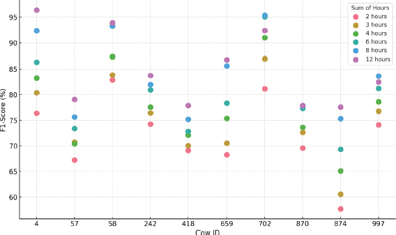
Figure 12. K-NN F1-Score results for each cow and hours considered
5.1.4. Minimum spanning tree results
The results obtained by applying MST to each data subset are presented in Table 4, which shows the configuration that yielded the best results among all those evaluated.
Table 4. MST results
Cow ID |
Hours considered |
Normalization |
Outlier fraction |
F1-Score (%) |
Standard deviation (%) |
4 |
2 |
NoNorm |
0.05 |
75.57 |
1.58 |
4 |
3 |
NoNorm |
0.05 |
80.70 |
3.93 |
4 |
4 |
NoNorm |
0.05 |
83.24 |
3.13 |
4 |
6 |
NoNorm |
0 |
85.09 |
1.85 |
4 |
8 |
NoNorm |
0 |
91.73 |
0.00 |
4 |
12 |
NoNorm |
0 |
95.10 |
1.23 |
57 |
2 |
NoNorm |
0.05 |
65.54 |
4.55 |
57 |
3 |
NoNorm |
0.05 |
69.97 |
7.35 |
57 |
4 |
NoNorm |
0.05 |
72.02 |
4.42 |
57 |
6 |
NoNorm |
0.05 |
71.94 |
4.30 |
57 |
8 |
Zscore |
0.05 |
74.63 |
5.71 |
57 |
12 |
NoNorm |
0.05 |
79.06 |
2.37 |
58 |
2 |
NoNorm |
0.05 |
85.30 |
2.24 |
58 |
3 |
NoNorm |
0.05 |
84.78 |
1.73 |
58 |
4 |
NoNorm |
0.05 |
87.46 |
2.80 |
58 |
6 |
NoNorm |
0 |
91.81 |
0.07 |
58 |
8 |
NoNorm |
0 |
90.84 |
1.37 |
58 |
12 |
NoNorm |
0 |
92.39 |
0.51 |
242 |
2 |
NoNorm |
0.05 |
76.38 |
3.61 |
242 |
3 |
Zscore |
0.05 |
76.03 |
2.45 |
242 |
4 |
NoNorm |
0.05 |
78.92 |
3.56 |
242 |
6 |
Zscore |
0.05 |
82.53 |
2.83 |
242 |
8 |
Norm |
0.05 |
82.34 |
2.18 |
242 |
12 |
Norm |
0.05 |
85.68 |
2.83 |
418 |
2 |
NoNorm |
0.05 |
70.74 |
5.12 |
418 |
3 |
NoNorm |
0.05 |
70.20 |
3.43 |
418 |
4 |
NoNorm |
0.05 |
74.81 |
3.99 |
418 |
6 |
Zscore |
0.05 |
73.07 |
3.95 |
418 |
8 |
NoNorm |
0.05 |
72.53 |
3.87 |
418 |
12 |
Zscore |
0.05 |
79.31 |
1.73 |
659 |
2 |
NoNorm |
0.05 |
69.04 |
4.24 |
659 |
3 |
NoNorm |
0.05 |
71.46 |
6.49 |
659 |
4 |
NoNorm |
0.05 |
71.74 |
2.68 |
659 |
6 |
NoNorm |
0.05 |
74.44 |
3.20 |
659 |
8 |
NoNorm |
0 |
79.87 |
0.99 |
659 |
12 |
NoNorm |
0 |
81.49 |
2.17 |
702 |
2 |
NoNorm |
0.05 |
81.05 |
3.19 |
702 |
3 |
NoNorm |
0.05 |
84.42 |
4.17 |
702 |
4 |
NoNorm |
0.05 |
86.97 |
2.91 |
702 |
6 |
NoNorm |
0 |
91.47 |
1.65 |
702 |
8 |
NoNorm |
0 |
92.65 |
1.64 |
702 |
12 |
NoNorm |
0 |
90.92 |
2.42 |
870 |
2 |
NoNorm |
0.1 |
62.43 |
2.87 |
870 |
3 |
NoNorm |
0.1 |
69.32 |
1.63 |
870 |
4 |
NoNorm |
0.1 |
69.62 |
3.34 |
870 |
6 |
NoNorm |
0.05 |
74.35 |
1.94 |
870 |
8 |
NoNorm |
0.05 |
73.22 |
0.83 |
870 |
12 |
NoNorm |
0.05 |
73.96 |
1.74 |
874 |
2 |
NoNorm |
0.05 |
50.90 |
4.99 |
874 |
3 |
NoNorm |
0.05 |
57.85 |
3.09 |
874 |
4 |
NoNorm |
0.05 |
69.06 |
5.45 |
874 |
6 |
NoNorm |
0.05 |
68.83 |
2.79 |
874 |
8 |
NoNorm |
0.05 |
71.46 |
2.51 |
874 |
12 |
NoNorm |
0 |
75.85 |
0.85 |
997 |
2 |
NoNorm |
0.05 |
76.90 |
3.41 |
997 |
3 |
NoNorm |
0.05 |
76.42 |
2.14 |
997 |
4 |
NoNorm |
0.05 |
42.70 |
2.86 |
997 |
6 |
NoNorm |
0 |
80.96 |
1.47 |
997 |
8 |
NoNorm |
0.05 |
81.10 |
1.69 |
997 |
12 |
NoNorm |
0.05 |
83.20 |
2.21 |
From the analysis of Table 4, the following observations are drawn:
•In general, the best MST results were achieved by using an outlier fraction of 0.05 and without applying data normalization.
•Evaluating this technique on the different datasets, a significant variability in performance is observed, with F1 Scores ranging from 42.7 % to 95.1 %, highlighting the sensitivity of MST to the specific characteristics of each dataset.
•As with previous techniques, MST performance varies considerably by animal and time interval analyzed. This pattern of variability can be seen graphically in Figure 13, which illustrates the differences between configurations and animals.
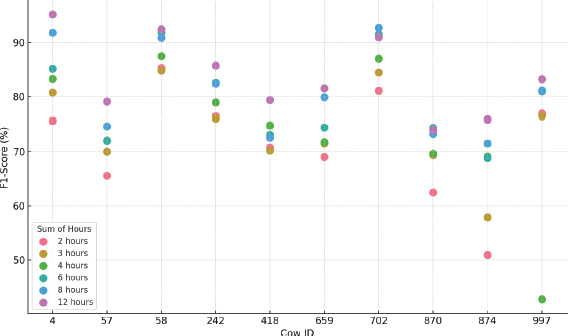
Figure 13. MST F1-Score results for each cow and hours considered
5.1.5. Approximate convex hull results
The ACH results, presented in Table 5, reflect the configuration that obtained the best results for each data subset. The following conclusions can be derived from this table:
•For ACH, lambda values of 1.2 and 1.4 tend to produce the best results, while the number of projections varies widely depending on the dataset. However, the best performance is achieved without data normalization.
•The F1-Score performance fluctuates significantly, with values between 40.5 % and 96.6 %, showing that this technique is highly dependent on the structure of the specific dataset. The variability in the results is marked both between animals and between time intervals. Figure 14 represents this dispersion in the results.
Table 5. ACH results
Cow ID |
Hours considered |
Normalization |
Lambda |
Number of projections |
F1-Score (%) |
Standard deviation (%) |
4 |
2 |
NoNorm |
1.2 |
1000 |
69.30 |
0.83 |
4 |
3 |
NoNorm |
1 |
800 |
78.09 |
0.44 |
4 |
4 |
NoNorm |
1.2 |
400 |
86.18 |
0.84 |
4 |
6 |
NoNorm |
1.4 |
800 |
92.61 |
0.51 |
4 |
8 |
NoNorm |
1 |
100 |
95.59 |
0.25 |
4 |
12 |
NoNorm |
1.4 |
600 |
96.02 |
0.37 |
57 |
2 |
NoNorm |
0.8 |
1000 |
31.63 |
4.79 |
57 |
3 |
NoNorm |
0.8 |
400 |
41.51 |
9.47 |
57 |
4 |
NoNorm |
0.8 |
600 |
21.38 |
4.83 |
57 |
6 |
NoNorm |
1.4 |
1000 |
56.13 |
2.32 |
57 |
8 |
NoNorm |
1 |
1000 |
62.66 |
1.49 |
57 |
12 |
NoNorm |
1.2 |
1000 |
51.27 |
1.92 |
58 |
2 |
NoNorm |
0.8 |
1000 |
79.18 |
2.21 |
58 |
3 |
NoNorm |
1 |
1000 |
90.27 |
0.81 |
58 |
4 |
NoNorm |
1 |
1000 |
92.49 |
0.31 |
58 |
6 |
NoNorm |
0.8 |
400 |
93.28 |
0.25 |
58 |
8 |
NoNorm |
1 |
1000 |
94.67 |
0.24 |
58 |
12 |
NoNorm |
1.2 |
200 |
94.85 |
0.18 |
242 |
2 |
NoNorm |
0.8 |
1000 |
56.22 |
3.13 |
242 |
3 |
NoNorm |
1.2 |
1000 |
61.47 |
3.98 |
242 |
4 |
NoNorm |
1.4 |
1000 |
74.47 |
1.99 |
242 |
6 |
NoNorm |
1.4 |
1000 |
81.79 |
0.64 |
242 |
8 |
NoNorm |
1.4 |
1000 |
82.60 |
0.93 |
242 |
12 |
NoNorm |
1.4 |
800 |
82.84 |
0.28 |
418 |
2 |
NoNorm |
1 |
1000 |
52.87 |
1.23 |
418 |
3 |
NoNorm |
1.4 |
1000 |
62.89 |
1.01 |
418 |
4 |
NoNorm |
0.8 |
1000 |
72.48 |
0.82 |
418 |
6 |
NoNorm |
1.2 |
400 |
69.27 |
0.29 |
418 |
8 |
NoNorm |
1 |
800 |
74.11 |
1.26 |
418 |
12 |
NoNorm |
1 |
1000 |
77.35 |
0.59 |
659 |
2 |
NoNorm |
1.4 |
1000 |
55.31 |
3.16 |
659 |
3 |
NoNorm |
0.8 |
1000 |
61.21 |
2.21 |
659 |
4 |
NoNorm |
1.2 |
800 |
73.99 |
1.87 |
659 |
6 |
NoNorm |
1.4 |
1000 |
80.21 |
0.46 |
659 |
8 |
NoNorm |
1.4 |
1000 |
82.66 |
2.40 |
659 |
12 |
NoNorm |
1.4 |
600 |
86.55 |
0.71 |
702 |
2 |
NoNorm |
0.8 |
1000 |
84.51 |
0.75 |
702 |
3 |
NoNorm |
1 |
1000 |
90.94 |
0.28 |
702 |
4 |
NoNorm |
1 |
1000 |
93.72 |
0.32 |
702 |
6 |
NoNorm |
1.4 |
600 |
95.80 |
0.29 |
702 |
8 |
NoNorm |
1.2 |
200 |
96.28 |
0.17 |
702 |
12 |
NoNorm |
1.2 |
1000 |
96.55 |
0.32 |
870 |
2 |
NoNorm |
1.4 |
800 |
40.48 |
1.00 |
870 |
3 |
NoNorm |
1 |
600 |
52.48 |
2.11 |
870 |
4 |
NoNorm |
1.4 |
1000 |
57.31 |
0.97 |
870 |
6 |
NoNorm |
1 |
1000 |
68.78 |
0.82 |
870 |
8 |
NoNorm |
1 |
1000 |
70.85 |
0.23 |
870 |
12 |
NoNorm |
1 |
1000 |
74.72 |
0.35 |
874 |
2 |
NoNorm |
1.4 |
1000 |
47.69 |
1.70 |
874 |
3 |
NoNorm |
1.2 |
1000 |
51.97 |
3.67 |
874 |
4 |
NoNorm |
1 |
600 |
60.55 |
1.18 |
874 |
6 |
NoNorm |
1.2 |
1000 |
74.13 |
1.28 |
874 |
8 |
NoNorm |
0.8 |
800 |
80.01 |
1.27 |
874 |
12 |
NoNorm |
1.4 |
200 |
83.28 |
0.42 |
997 |
2 |
NoNorm |
1.2 |
1000 |
62.22 |
2.13 |
997 |
3 |
NoNorm |
1 |
1000 |
76.75 |
1.12 |
997 |
4 |
NoNorm |
1.2 |
1000 |
81.91 |
0.85 |
997 |
6 |
NoNorm |
1.2 |
800 |
83.60 |
0.56 |
997 |
8 |
NoNorm |
1.2 |
800 |
84.92 |
0.41 |
997 |
12 |
NoNorm |
1 |
1000 |
86.33 |
0.30 |
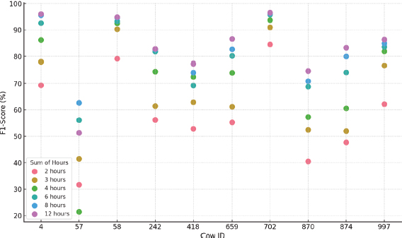
Figure 14. ACH F1-Score results for each cow and hours considered
5.1.6. Non-convex boundary over projection results
Finally, the results of the NCBoP technique are detailed in Table 6. The following conclusions can be drawn from these results:
•The NCBoP technique shows similar overall patterns to ACH, with better results using lambda values of 1.4, although in some cases (8 instances) a lambda of 1.2 proved to be more effective. As with ACH, normalization does not appear to enhance performance, as the strongest results were achieved without data normalization.
•F1 Score values for NCBoP range from 53.4 % to 97.5 %, revealing a considerable variability that suggests the influence of the particular characteristics of each dataset and of individual animal behavior patterns on the precision of the model. These differences are clearly illustrated in Figure 15.
Table 6. NCBoP results
Cow ID |
Hours considered |
Normalization |
Lambda |
Number of projections |
F1-Score (%) |
Standard deviation (%) |
4 |
2 |
NoNorm |
1.4 |
200 |
83.88 |
3.33 |
4 |
3 |
NoNorm |
1.4 |
600 |
85.17 |
2.50 |
4 |
4 |
NoNorm |
1.4 |
200 |
89.92 |
1.75 |
4 |
6 |
NoNorm |
1.4 |
200 |
94.63 |
1.16 |
4 |
8 |
NoNorm |
1.4 |
10 |
94.57 |
0.62 |
4 |
12 |
NoNorm |
1.4 |
10 |
94.68 |
1.57 |
57 |
2 |
Norm |
1.4 |
1000 |
65.53 |
5.73 |
57 |
3 |
Norm |
1.4 |
600 |
74.13 |
5.86 |
57 |
4 |
NoNorm |
1.4 |
1000 |
82.25 |
6.28 |
57 |
6 |
NoNorm |
1.4 |
1000 |
87.49 |
5.80 |
57 |
8 |
NoNorm |
1.4 |
400 |
89.24 |
2.30 |
57 |
12 |
NoNorm |
1.4 |
800 |
89.40 |
1.89 |
58 |
2 |
NoNorm |
1.4 |
1000 |
90.91 |
0.72 |
58 |
3 |
NoNorm |
1.4 |
1000 |
92.43 |
1.30 |
58 |
4 |
NoNorm |
1.4 |
100 |
92.16 |
2.52 |
58 |
6 |
NoNorm |
1.4 |
10 |
92.88 |
0.79 |
58 |
8 |
NoNorm |
1.4 |
50 |
93.95 |
0.76 |
58 |
12 |
NoNorm |
1.4 |
200 |
94.50 |
0.77 |
242 |
2 |
NoNorm |
1.4 |
1000 |
75.61 |
4.32 |
242 |
3 |
NoNorm |
1.4 |
1000 |
81.07 |
3.27 |
242 |
4 |
NoNorm |
1.4 |
1000 |
86.24 |
3.11 |
242 |
6 |
NoNorm |
1.4 |
1000 |
88.99 |
1.99 |
242 |
8 |
NoNorm |
1.4 |
400 |
88.81 |
1.73 |
242 |
12 |
Zscore |
1.4 |
200 |
89.26 |
2.30 |
418 |
2 |
Zscore |
1.4 |
1000 |
62.70 |
4.45 |
418 |
3 |
NoNorm |
1.4 |
1000 |
71.80 |
3.73 |
418 |
4 |
NoNorm |
1.4 |
200 |
75.84 |
4.41 |
418 |
6 |
NoNorm |
1.4 |
1000 |
79.27 |
3.89 |
418 |
8 |
NoNorm |
1.4 |
800 |
78.72 |
2.97 |
418 |
12 |
NoNorm |
1.4 |
400 |
81.36 |
2.09 |
659 |
2 |
NoNorm |
1.4 |
600 |
73.19 |
3.25 |
659 |
3 |
NoNorm |
1.4 |
1000 |
81.59 |
2.24 |
659 |
4 |
NoNorm |
1.4 |
200 |
84.40 |
5.12 |
659 |
6 |
NoNorm |
1.4 |
50 |
83.91 |
2.99 |
659 |
8 |
NoNorm |
1.4 |
100 |
87.34 |
2.46 |
659 |
12 |
NoNorm |
1.4 |
100 |
85.80 |
1.47 |
702 |
2 |
NoNorm |
1.4 |
400 |
86.73 |
1.88 |
702 |
3 |
NoNorm |
1.4 |
400 |
91.79 |
1.54 |
702 |
4 |
NoNorm |
1.4 |
50 |
93.44 |
2.36 |
702 |
6 |
NoNorm |
1.4 |
10 |
95.18 |
1.05 |
702 |
8 |
NoNorm |
1.4 |
50 |
95.89 |
0.83 |
702 |
12 |
NoNorm |
1.4 |
10 |
97.48 |
0.75 |
870 |
2 |
NoNorm |
1.2 |
600 |
60.45 |
1.37 |
870 |
3 |
NoNorm |
1.2 |
800 |
65.93 |
1.77 |
870 |
4 |
NoNorm |
1.4 |
600 |
69.72 |
1.08 |
870 |
6 |
Zscore |
1.4 |
800 |
72.11 |
1.94 |
870 |
8 |
NoNorm |
1.4 |
200 |
74.97 |
2.47 |
870 |
12 |
NoNorm |
1.2 |
400 |
75.91 |
2.02 |
874 |
2 |
NoNorm |
1.2 |
50 |
53.37 |
5.18 |
874 |
3 |
Zscore |
1.2 |
50 |
56.35 |
2.87 |
874 |
4 |
NoNorm |
1.2 |
10 |
63.76 |
1.69 |
874 |
6 |
NoNorm |
1.4 |
50 |
74.08 |
4.89 |
874 |
8 |
NoNorm |
1.2 |
10 |
78.10 |
1.80 |
874 |
12 |
NoNorm |
1.2 |
10 |
78.13 |
1.78 |
997 |
2 |
NoNorm |
1.4 |
600 |
75.13 |
1.18 |
997 |
3 |
NoNorm |
1.4 |
400 |
82.37 |
2.19 |
997 |
4 |
Norm |
1.4 |
800 |
83.87 |
2.35 |
997 |
6 |
NoNorm |
1.4 |
50 |
83.91 |
2.27 |
997 |
8 |
NoNorm |
1.4 |
200 |
85.95 |
1.35 |
997 |
12 |
NoNorm |
1.4 |
400 |
86.91 |
2.24 |

Figure 15. NCBoP F1-Score results for each cow and hours considered
5.2. Comparative analysis of results
Once the one-class techniques were analyzed individually, a detailed analysis was performed for each animal, as well as for the hours considered for the generation of the new variables, following the procedure described in Section 4.2.
The aim of this analysis is to identify significant differences in the results obtained for each animal and to determine which temporal data window offers the best performance in the detection of behavioral patterns related to estrus.
Following two key graphs for this analysis:
•Figure 16 provides a line graph representing, from among all the techniques implemented, the best F1-Score value achieved for each cow and for each hour interval. Each line of the graph, represented with a different color, corresponds to a specific cow.
•Figure 17 presents a boxplot that summarizes the results obtained with each technique and configuration of hours considered. In this graph, each color represents a different hour configuration.
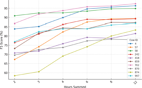
Figure 16. Line graph showing the best results obtained for each cow according to the hours considered
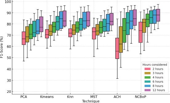
Figure 17. Boxplot grouped by technique and configuration of hours considered
Analyzing Figure 16, it can be observed that the results differ considerably among the cows. In particular, the models generated for cows 702, 4 and 58 showed a higher performance than the rest of the animals, reaching F1-Score values above 95 % in their best configurations. In contrast, the model generated with data from cow 870 showed a maximum performance slightly above 78 %. As discussed in the technique-by-technique analysis, such significant variation among animals suggests that behavioral patterns differ greatly among cows.
This significant variations in the results obtained for each animal may be due to several reasons. First, the data recorded in certain animals may have more noise due to inaccurate placement of the smart collar, which directly affects the accuracy and identification of the different behaviors monitored. On the other hand, it is possible that, due to the difficulty in the data tagging process, small inaccuracies may have been committed, which impacts on the data quality. Finally, some animals may exhibit less well-defined behavioral patterns in both normal activity and estrus behavior, making it more difficult to detect this event early. Therefore, to improve performance, it is essential to develop individual animal model.
Furthermore, in the same graph (Figure 16), it can be noted that, for all cows, considering a higher number of hours significantly improves the performance of the model in terms of F1-Score. In the best performing animals, the results improve after considering six or more hours, reaching the maximum in almost all animals when considering 12 hours. Thus, it can be concluded that in order to accurately detect cow estrus, it is essential to provide temporal context to the model. This is because estrus represents a change in the animal's behavioral pattern over several hours.
Finally, analyzing the results shown in Figure 17, the conclusions obtained in the previous graph (Figure 16) are corroborated. In addition, it can be determined that, in general terms, the technique that showed the best results was NCBoP together with ACH, using the configurations that considered a greater number of hours. In contrast, the technique that presented the worst performance was PCA.
6. Conclusions and future work
This paper presents a novel intelligent system based on the use of one-class techniques for the early detection of estrus in cattle on intensive dairy farms. The system monitors the behavior of the animals from the data provided by an intelligent collar. In this research work, the monitoring collar RUMI, developed by the Galician startup Innogando, has been used. This device not only allows GPS location, but also the monitoring of key activities such as rumination or resting time, among others.
For this research work, data was collected from a total of 10 Holstein Friesian cows from an intensive dairy farm over a period of 95 days. These cows comprised different ages, which added diversity to the behavioral sample. Feature engineering techniques were applied to the collected data in order to increase the dataset variables; new attributes were added, reflecting the accumulation of each behavior recorded at time intervals ranging from 2, 3, 4, 6, 8 and 12 hours. This aggregation process was implemented to provide greater temporal context to the models’ inputs. For each of the hourly configurations, the performance of six different one-class techniques was evaluated, developing individualized models for each animal.
The obtained results have shown a high variability in model performance among different animals, suggesting that the behavioral patterns related to estrus vary significantly between cows.
Among the implemented techniques, NCBoP and ACH were the most effective, reaching the highest F1-scores, with values higher than 95 % F1-Score when longer time intervals were considered for the generation of the new variables. In contrast, PCA presented the worst overall performance.
In general terms, it can be highlighted how the use of time windows that accumulate behaviors in intervals of more than 6 hours significantly improved the performance of the models, highlighting the importance of the temporal context for accurate heat behavior detection.
In summary, this study highlights the need to develop individualized models per animal to improve accuracy in heat detection due to observed differences in behavioral patterns among cows. Providing greater temporal context has also proven to be a critical factor in improving results in the classification of estrus-related behaviors.
The presented proposal provides a valuable tool for efficient herd management, contributing to efficient heat detection, which can significantly increase gestation success rates.
Although the results obtained have been highly satisfactory, the need to develop individualized models per animal represents a significant challenge. This approach involves a customized model setup for each animal, which can be complex on farms where many cows need to be monitored. The additional workload to calibrate and maintain animal-specific models could limit the scalability and efficient use of this methodology on large farms and suggests the need to explore alternatives or adaptations that facilitate a more efficient implementation.
As future work, further tests are planned with larger datasets, including a larger number of cows, as well as recording behaviors in cows from other farms and herds. In addition, the performance of one-class methods implemented on extensive farms will be explored.
Acknowledgments
Álvaro Michelena’s research was supported by the Spanish Ministry of Universities (https://www.universidades.gob.es/), under the “Formación de Profesorado Universitario” grant with reference FPU21/00932.
Xunta de Galicia. Grants for consolidating and structuring competitive research units, GPC (ED431B 2023/49).
CITIC, as a center accredited for excellence within the Galician University System and a member of the CIGUS Network, receives subsidies from the Department of Education, Science, Universities, and Vocational Training of the Xunta de Galicia. Additionally, it is co-financed by the EU through the FEDER Galicia 2021-27 operational program (Ref. ED431G 2023/01).
The dataset has been provided by the Galician startup Innogando.
References
Abu Alfeilat, H. A., Hassanat, A. B., Lasassmeh, O., Tarawneh, A. S., Alhasanat, M. B., Eyal Salman, H. S., & Prasath, V. S. (2019). Effects of distance measure choice on k-nearest neighbor classifier performance: A review. Big data, 7(4), 221–248.
Alonso, M. E., Gonzalez-Montana, J. R., & Lomillos, J. M. (2020). Consumers’ concerns and perceptions of farm animal welfare. Animals, 10(3), 385.
Al-Qudah, M., Ashi, Z., Alnabhan, M., & Abu Al-Haija, Q. (2023). Effective one-class classifier model for memory dump malware detection. Journal of Sensor and Actuator Networks, 12(1), 5.
Annas, M., & Wahab, S. N. (2023). Data mining methods: K-means clustering algorithms. International Journal of Cyber and IT Service Management, 3(1), 40–47.
Bansal, M., Goyal, A., & Choudhary, A. (2022). A comparative analysis of k-nearest neighbor genetic, support vector machine, decision tree, and long short term memory algorithms in machine learning. Decision Analytics Journal, 3, 100071.
Bruyere, P., Hetreau, T., Ponsart, C., Gatien, J., Buff, S., Disenhaus, C., Giroud, O., & Guerin, P.(2012). Can video cameras replace visual estrus detection in dairy cows? Theriogenology, 77(3), 525–530.
Carvajal, A., Martinez, E., Tapia, M., & Ayke, I. T. (2020). El ciclo estral en la hembra bovina y su importancia productiva. Instituto de investigaciones agropecuarias, 246, 1–4.
Casale, P., Pujol, O., & Radeva, P. (2011). Approximate convex hulls family for one-class classification. Multiple Classifier Systems: 10th International Workshop, MCS 2011,
Cocco, R., Canozzi, M. E. A., & Fischer, V. (2021). Rumination time as an early predictor of metritis and subclinical ketosis in dairy cows at the beginning of lactation: Systematic review-meta-analysis. Preventive Veterinary Medicine, 189, 105309.
Fernandez-Francos, D., Fontenla-Romero, O., & Alonso-Betanzos, A. (2017). One-class convex hull-based algorithm for classification in distributed environments. IEEE Transactions on Systems, Man, and Cybernetics: Systems, 50(2), 386–396.
Fesseha, H., & Degu, T. (2020). Estrus detection, estrus synchronization in cattle and it’s economic importance. Int. J. Vet. Res, 3(1), 1001.
Fogsgaard, K. K., Bennedsgaard, T. W., & Herskin, M. S. (2015). Behavioral changes in freestall-housed dairy cows with naturally occurring clinical mastitis. Journal of dairy science, 98(3), 1730–1738.
Fukase, E., & Martin, W. (2020). Economic growth, convergence, and world food demand and supply. World Development, 132, 104954. https://doi.org/10.1016/j.worlddev.2020.104954
Garcia, R., Aguilar, J., Toro, M., Pinto, A., & Rodriguez, P. (2020). A systematic literature review on the use of machine learning in precision livestock farming. Computers and Electronics in Agriculture, 179, 105826.
Gautam, G. (2023). Postpartum anestrus in dairy cattle and its management. AIP Conference Proceedings, 2628(1).
Rayas-Amor, Adolfo & Espinoza, A. & Arriaga-Jordán, Carlos & Mould, F. & Castelan-Ortega, Octavio. (2005). Grassland: a global resource. https://doi.org/10.3920/978-90-8686-551-2
Greenacre, M., Groenen, P. J., Hastie, T., d’Enza, A. I., Markos, A., & Tuzhilina, E. (2022). Principal component analysis. Nature Reviews Methods Primers, 2(1), 100.
Hu, H., Liu, J., Zhang, X., & Fang, M. (2023). An effective and adaptable k-means algorithm for big data cluster analysis. Pattern Recognition, 139, 109404.
Jabbar, W. A., Subramaniam, T., Ong, A. E., Shu’Ib, M. I., Wu, W., & De Oliveira, M. A. (2022). Lorawan-based iot system implementation for long-range outdoor air quality monitoring. Internet of Things, 19, 100540.
Jove, E., Casteleiro-Roca, J.-L., Quintian, H., Mendez-Perez, J.-A., & Calvo-Rolle, J. L. (2021). A new method for anomaly detection based on non-convex boundaries with random two-dimensional projections. Information Fusion, 65, 50–57.
Juszczak, P., Tax, D. M., Pe, kalska, E., & Duin, R. P. (2009). Minimum spanning tree based one-class classifier [Advances in Machine Learning and Computational Intelligence]. Neurocomputing, 72(7), 1859–1869. https://doi.org/10.1016/j.neucom.2008.05.003
La Grassa, R., Gallo, I., & Landro, N. (2022). Ocmst: One-class novelty detection using convolutional neural network and minimum spanning trees. Pattern Recognition Letters, 155, 114–120.
Ma, N., Pan, L., Chen, S., & Liu, B. (2020). Nb-iot estrus detection system of dairy cows based on lstm networks. 2020 IEEE 31st Annual International Symposium on Personal, Indoor and Mobile Radio Communications, 1–5.
Michelena, A., Fontenla-Romero, O., & Luis Calvo-Rolle, J. (2024). A review and future trends of precision livestock over dairy and beef cow cattle with artificial intelligence. Logic Journal of the IGPL, jzae111. https://doi.org/10.1093/jigpal/jzae111
Morrone, S., Dimauro, C., Gambella, F., & Cappai, M. G. (2022). Industry 4.0 and precisión livestock farming (plf): An up to date overview across animal productions. Sensors, 22(12), 4319.
Neethirajan, S. (2020). The role of sensors, big data and machine learning in modern animal farming. Sensing and Bio-Sensing Research, 29, 100367.
Niloofar, P., Francis, D. P., Lazarova-Molnar, S., Vulpe, A., Vochin, M.-C., Suciu, G., Balanescu, M., Anestis, V., & Bartzanas, T. (2021). Data-driven decision support in livestock farming for improved animal health, welfare and greenhouse gas emissions: Overview and challenges. Computers and Electronics in Agriculture, 190, 106406.
Pratama, Y. P., Basuki, D. K., Sukaridhoto, S., Yusuf, A. A., Yulianus, H., Faruq, F., & Putra, F. B. (2019). Designing of a smart collar for dairy cow behavior monitoring with application monitoring in microservices and internet of things-based systems. 2019 International Electronics Symposium (IES), 527–533.
Raschka, S. (2014). An overview of general performance metrics of binary classifier systems. arXiv preprint arXiv:1410.5330.
Reith, S., & Hoy, S. (2018). Behavioral signs of estrus and the potential of fully automated systems for detection of estrus in dairy cattle. Animal, 12(2), 398–407.
Riaz, U., Idris, M., Ahmed, M., Ali, F., & Yang, L. (2023). Infrared thermography as a potential non-invasive tool for estrus detection in cattle and buffaloes. Animals, 13(8), 1425.
Roelofs, J., Van Eerdenburg, F., Soede, N., & Kemp, B. (2005). Various behavioral signs of estrous and their relationship with time of ovulation in dairy cattle. Theriogenology, 63(5), 1366–1377.
Roelofs, J., Lopez-Gatius, F., Hunter, R., Van Eerdenburg, F., & Hanzen, C. (2010). When is a cow in estrus? clinical and practical aspects. Theriogenology, 74(3), 327–344.
Ruviaro, C. F., de Leis, C. M., Florindo, T. J., de Medeiros Florindo, G. I. B., da Costa, J. S.,Tang, W. Z., Pinto, A. T., & Soares, S. R. (2020). Life cycle cost analysis of dairy production systems in southern Brazil. Science of the Total Environment, 741, 140273.
Scott, D. W. (2015). Multivariate density estimation: Theory, practice, and visualization. John Wiley & Sons.
Silper, B., Madureira, A., Kaur, M., Burnett, T., & Cerri, R. (2015). Comparison of estrus characteristics in holstein heifers by 2 activity monitoring systems. Journal of dairy science, 98(5), 3158–3165.
Sinaga, K. P., & Yang, M.-S. (2020). Unsupervised k-means clustering algorithm. IEEE access, 8, 80716–80727.
Tax, D. M. J. (2001). One-class classification: Concept-learning in the absence of counter-examples [ph. d. thesis]. Delft University of Technology.
Tax, D. (2018, January). Ddtools, the data description toolbox for matlab [version 2.1.3].
Thanh, L. T., Nishikawa, R., Takemoto, M., Binh, H. T. T., & Nakajo, H. (2018). Cow estrus detection via discrete wavelet transformation and unsupervised clustering. Proceedings of the 9th International Symposium on Information and Communication Technology, 305–312.
Thornton, P. K. (2010). Livestock production: Recent trends, future prospects. Philosophical Transactions of the Royal Society B: Biological Sciences, 365(1554), 2853–2867. https://doi.org/10.1098/rstb.2010.0134
Wang, J., Bell, M., Liu, X., & Liu, G. (2020). Machine-learning techniques can enhance dairy cow estrus detection using location and acceleration data. Animals, 10(7), 1160.
Zhang, X., & Liu, C.-A. (2023). Model averaging prediction by k-fold cross-validation. Journal of Econometrics, 235(1), 280–301.
Zhang, Z. (2016). Introduction to machine learning: K-nearest neighbors. Annals of translational medicine, 4(11).
Zheng, A., & Casari, A. (2018). Feature engineering for machine learning: Principles and techniques for data scientists. O’Reilly Media, Inc.