ADCAIJ: Advances in Distributed Computing and Artificial Intelligence Journal
Regular Issue, Vol. 13 (2024), e31866
eISSN: 2255-2863
DOI: https://doi.org/10.14201/adcaij.31866
Bus Ridership Prediction and Scenario Analysis through ML and Multi-Agent Simulations
Pasqual Martía, Alejandro Ibáñeza, Vicente Juliana,b, Paulo Novaisc and Jaume Jordána
a Valencian Research Institute for Artificial Intelligence (VRAIN), Universitat Politècnica de València, Valencia, Spain
b Valencian Graduate School and Research Network of Artificial Intelligence, Universitat Politècnica de València,
Valencia, Spain
c ALGORITMI Centre, Universidade do Minho, Braga, Portugal
✉ pasmargi@vrain.upv.es, alejandro.ibapen@gmail.com, vjulian@upv.es, pjon@di.uminho.pt, jjordan@dsic.upv.es
ABSTRACT
This paper introduces an innovative approach to predicting bus ridership andanalysing transportation scenarios through a fusion of machine learning (ML) techniques and multi-agent simulations. Utilising a comprehensive dataset from an urban bus system, we employ ML models to accurately forecast passenger flows, factoring in diverse variables such as weather conditions. The novelty of our method lies in the application of these predictions to generate detailed simulation scenarios, which are meticulously executed to evaluate the efficacy of public transportation services. Our research uniquely demonstrates the synergy between ML predictions and agent-based simulations, offering a robust tool for optimising urban mobility. The results reveal critical insights into resource allocation, service efficiency, and potential improvements in public transport systems. This study significantly advances the field by providing a practical framework for transportation providers to optimise services and address long-term challenges in urban mobility
KEYWORDS
Passenger prediction; Urban mobility; Agent simulation
1. Introduction
Public transportation is a crucial necessity globally. According to statistics1, in the United States, 12 % of the population relies on public transport daily, while countries such as South Korea have reached 40 %. Accurately predicting bus occupancy levels is key to optimising routes, enhancing reliability, and reducing waiting times. Historical data allows to proactively identify issues such as bottlenecks, rush hour shortages, and resource wastage. Modifying route planning and resource allocation based on these insights can prevent problems and improve public transportation systems.
This paper aims to establish a benchmark for public transportation systems, to analyse their performance across various environments and identify long-term challenges through experimental simulation. The main contribution of this work is the creation of an initial passenger demand with a specific environmental setup, its load to a fleet simulator, and the analysis of the simulations themselves. To achieve this, traditional and machine learning (ML) techniques were employed to develop models that accurately predict bus occupancy levels, whereas multi-agent simulation was used to validate the predictions. Our approach’s performance was evaluated using a real-world bus system dataset.
Bus passenger flow optimisation has been a widely discussed topic in recent years. Studies by (Baghbani et al., 2023) and (Nagaraj et al., 2022) achieve a real-time passenger prediction task using a final Long Short-Term Memory (LSTM) model layer (Schmidhuber and Hochreiter, 1997). Such a technique can not be directly applied to the current work since the simulation requires an atemporal prediction, but it may be useful for our study to use a modification. Similarly, the study by (Liyanage et al., 2022) employed a bidirectional LSTM model for atemporal prediction, obtaining satisfactory results. Nevertheless, the technique is unsuitable for our purpose, as in a real-scenario application of a simulation, future data would not be available, thus sticking to the unidirectional part of the model.
Moreover, research by (Ming et al., 2014) used a combination of ARIMA-SVM models, where the first one captured the linearity of the data, while the other, the non-linearity. Lastly, (Zhang et al., 2017) used a Grey Prediction Model (GM) (Julong et al., 1989). GM models are widely used in passenger prediction since they capture two types of patterns: normal trends (from day to day) and cyclic trends (between the same weekday at different weeks). More traditional ML techniques can also be adequate for the passenger prediction task. Thus, techniques such as Random Forest (RF), Support Vector Machine for Regression (SVR), and Neural Network (NN) can produce good results depending on the context.
Recently, passenger ridership prediction has been used in transportation optimisation research to help decision- making for mass-transportation operators. The study by (Santanam et al., 2024) focuses on post-event (sports, concerts, etc.) ridership prediction combined. Their approach combines ML with historical trends to forecast the passenger flow curve at stations near the event, finally estimating transport frequencies to serve as many customers as possible. Similarly, the study of (AlKhereibi et al., 2023), approaches the same issue but adds the urban land use information and the built environment around the stations to enrich their prediction. Most recent studies use a variety of ML and traditional statistical techniques, such as the work by (Nair et al., 2023), thus maximising their optimisation options. RF and linear regression models provide, in general, good results in this area. However, more modern hybrid predictors may overcome traditional models for specific issues, as demonstrated by the experimentation of (Lv et al., 2024). Finally, it is worth mentioning that ridership prediction is often combined with anomaly detection, as exemplified by (He et al., 2022), better exploiting data to create more useful solutions.
In the specific context of bus passenger demand prediction, there are primarily two simulation methodologies that stand out for their effectiveness and applicability. The first is agent-based modelling (Hajinasab et al., 2016), which is an intricate approach where each bus and passenger is represented as an individual agent. These agents interact within a simulated environment, mirroring real-world dynamics. This method excels in capturing the complex behaviours and interactions among buses, passengers, and their surroundings. However, the detailed nature of agent-based models often makes them computationally intensive and reliant on extensive data inputs and careful parameter tuning.
The second notable methodology is discrete event simulation (Gunawan et al., 2014). This approach views the bus system’s operations as a series of discrete, time-stamped events. Each event represents a significant change within the system, such as a bus arriving at a stop or passengers boarding and alighting. Discrete event simulation is particularly adept at handling large-scale systems, offering a more streamlined and efficient way to model processes compared to agent-based models. However, its main limitation lies in potentially not capturing the full dynamic behaviour of bus systems, especially the nuanced interactions between the different elements of the system.
In our research, we have chosen to utilise agent-based simulation. This decision is grounded in the method’s superior ability to replicate the intricate dynamics of urban bus systems. By leveraging agent-based models combined with advanced machine learning techniques, we are able to generate realistic and detailed simulations of passenger demand and bus system operations. These simulations are crucial in analysing and understanding the performance and efficiency of the transportation service. Our application of agent-based simulation to a real-world urban bus service has provided valuable insights, demonstrating the model’s efficacy in informing decision-making processes for transportation providers and aiding in the development of optimised transportation services.
Our current research contributes to the development of practical applications for the analysis and enhancement of transportation services. On the one hand, the developed ML prediction models allow us to realistically generalise demand data for the studied transportation system. On the other hand, the predicted demand can be used to create realistic simulation scenarios that reproduce the transportation service in motion. The analysis of such simulations permits the discovery of trends in the performance of the transportation service. Our experimentation on a real-world urban bus service and the subsequent result analysis proves the usefulness of our approach when it comes to guiding the decision-making process of transportation providers, helping the configuration of an optimised service. This paper significantly extends the work presented by (Ibáñez et al., 2023) and builds on the earlier ideas set out in that work.
The rest of the paper is organised as follows: Section 2 describes the data and its treatment. Section 3 presents the training of the demand prediction models. The simulation data generation is described, alongside experimental results, in Section 4. Then, Section 5 goes over the contribution of the paper and the limitations of the chosen techniques. Lastly, Section 6 presents the conclusions and the future line of work.
2. Data
Over the past years, significant endeavours have been made to enhance public transportation systems. These endeavours often involve collecting and analysingvarious data sources to uncover patterns, trends, and valuable insights to support decision-making. This section describes the data fed to the ML techniques and the transformations applied to it for proper learning. A dataset provided by the Ames Transit Agency in Ames, Iowa, has been chosen, as it offers the most comprehensive information available on bus transportation in urban areas.
2.1. Data Sourcing
The bus occupancy data utilised in this study was obtained from multiple routes operated by the Ames Transit Agency in the metropolitan area of Ames, Iowa, spanning from October 2021 to June 2022 (Wilbur, 2022). In total, the dataset comprises 4,577,930 records. The data was collected using automatic passenger counters (APCs), ensuring that each entry in the database corresponds to the number of passengers boarding and alighting at each bus stop.
In addition to passenger counts, each record includes information about the route, scheduled and actual arrival and departure times, and the vehicle’s capacity. The bus routes consist of nine circular routes, three linear routes (with separate routes for outward and inward journeys), and one hybrid route (linear during the school year and circular during summer). Among these routes, four exhibit operational inconsistencies: one undergoes changes in its itinerary on weekdays and weekends, one has limited service resulting in periods of missing data, and two do not operate or have altered routes during the summer season. Therefore, in this study, we only considered nine routes that have consistent data, two of them being round-trip routes, so we will finally refer to the following eleven routes: 1E, 1W, 2E, 2W, 3, 5, 7, 9, 11, 14, and 23.
The dataset covers five different bus types, categorised according to passenger capacity. These types, ranked by usage frequency, are as follows: 60 passengers (70.02 %), 65 passengers (23.16 %), 90 passengers (4.84 %), 40 passengers (1.63 %), and 20 passengers (0.35 %).
2.2. Pre-Processing
Several steps were taken to unify the dataset for training. Firstly, routes displaying inconsistencies were excluded, preserving two linear (round-trip) routes and seven circular routes, as commented before. Also, during the data collection period, the stops of some routes were modified. To adapt the dataset, stops that no longer existed were removed, while new stops were disregarded. Finally, some routes had multiple patterns, as temporary alterations occurred during certain events. However, due to the time-sensitive nature of these cases, they were omitted from the dataset.
Since the aim of prediction is to estimate the number of passengers requiring bus services within a specific time range and area, the data, presented as individual records, needed to be aggregated into flows. This involved defining sections by grouping stops and establishing time ranges. Each route was divided using Ames neighbourhoods as a reference and then subdivided considering changes in the surroundings of a bus stop, such as transitioning from residential to commercial zones. The black rectangles in Figure 1 provide a visual representation of the section divisions.

Figure 1. Public bus routes in Ames, labelled by number and colour. Rectangular sections of the area represent divisions by groups of stops
Regarding time zones, the schedule of Iowa State University2 served as the basis for creating 7 time periods to account for fluctuations in passenger occupancy. Table 1, under «Time period division», describes each period. The night periods from the previous and current day were aggregated into a single period.
Table 1. Columns under «Time period division» describe the chosen time periods for passenger flow. Columns under «Precipitation» describe weighted windows for previous and current day precipitation. Finally, columns under «Snow depth» describe weighted windows for the current and following day’s snow depth.
Time period division |
Precipitation |
Snow depth |
||||
Period |
Starts |
Ends |
Prev. day |
Curr. day |
Curr. day |
Fol. day |
1_night |
22:00 (prev. day) |
4:59 |
5/6 |
1/6 |
6/6 |
0/6 |
2_early_morning |
5:00 |
8:59 |
4/6 |
2/6 |
5/6 |
1/6 |
3_morning |
9:00 |
11:59 |
3/6 |
3/6 |
4/6 |
2/6 |
4_midday |
12:00 |
14:59 |
2/6 |
4/6 |
3/6 |
3/6 |
5_afternoon |
15:00 |
18:59 |
1/6 |
5/6 |
2/6 |
4/6 |
6_evening |
19:00 |
21:59 |
0/6 |
6/6 |
1/6 |
5/6 |
As the occupancy rate in public transportation follows weekly trends (Liu et al., 2019), two additional variables were created to keep that context: «ons_yesterday» and «ons_last_week». «ons_yesterday» stores the total onboardings during the previous day at the same route, section and hour range, whereas «ons_last_week» does the same but for the previous week, on the same weekday. With this, both a general trend and a particular trend for each weekday were procured. Variables for offboarding were also created analogously.
The environmental conditions have some effect on the behaviour of passenger traffic in public transport (Wang et al., 2020). Therefore, in order to enhance the data analysis and investigate the impact of different weather conditions, a weather dataset was incorporated from the Iowa Environmental Mesonet3. The specific weather station selected for this study was AMES 5 SE, identified by the code IA0203. The weather data, however, had a different level of granularity compared to the existing dataset, as it provided daily information instead of hourly data. To overcome this disparity, weather values for each hour range were inferred by considering the adjacent days as a moving window. Rather than simply retaining the daily value or using a fraction of it, this approach ensured a more accurate estimation. Such a value was derived from a sixth of the weighted total data from the previous and current day. This methodology, as outlined in Table 1, under «Precipitation», accounted for precipitation trends and mitigated the impact of intense downpours.
On the other hand, for the snow depth variable, we considered the gradual melting of snow over time. A weighted average of the current day and the following day was calculated to estimate the snow depth value for each hour range. This approach is depicted in Table 1, under «Snow depth».
By incorporating the weather dataset and employing these inference techniques, the analysis could capture the influence of various meteorological conditions on the bus transportation system with greater accuracy and detail.
The final aggregation structure consists of the route as the first level, followed by the section, date, and time range, and includes the aforementioned information on onboadings, offboardings and weather conditions. Hence, the dataset and the description of each field can be seen in Table 2.
Table 2. Variable description. Onboarding-Offboarding dataset
Variable |
Description |
hour |
Time range. See Table 1. |
weekday |
Day of the week. |
day |
Day of the month. Kept only to order the dataset. |
month |
Month of the year. |
year |
Kept only to order the dataset. |
section |
Stops aggregation in each route. |
route_name |
Identifier of the different lanes in Ames’ bus transport. |
ons_yesterday |
Total onboarding during the previous day for a certain section within a certain route in a certain hour. Only for onboarding prediction. |
ons_last_week |
Total onboarding during the previous week at the same weekday for a certain section within a certain route in a certain hour. Only for onboarding prediction. |
offs_yesterday |
Total offboarding during the previous day for a certain section within a certain route in a certain hour. Only for offboarding prediction. |
offs_last_week |
Total offboarding during the previous week at the same weekday for a certain section within a certain route in a certain hour. Only for offboarding prediction. |
precip_mm |
Inferred total rain and melted snow precipitation during the same hour range of the previous day. |
snow |
Inferred total snow precipitation during the same hour range of the previous day. |
snow_d |
Inferred inches of accumulated snow for the same hour range of the previous day. |
ons |
Target variable. Accumulated quantity of individuals that get on the bus at any stop of a certain section. |
Offs |
Target variable. Accumulated quantity of individuals that get off the bus at any stop of a certain section. |
3. Model Training and Evaluation
The individuals in our data are treated as independent blocks without the context of previous time steps. However, considering real-world trends, we incorporate the daily and weekly boarding variables such as «ons_yesterday» and «ons_last_week» to provide contextual information on normal and periodic trends, respectively. The same process has been done for the offboarding models. We create separate models for each route to optimise efficiency rather than using a generalised model with a route variable decision-maker. This approach reduces convergence and prediction time.
For our approach, we employ Random Forest (RF), Support Vector Machine for Regression (SVR), and Neural Network (NN) techniques. It is also important to note that we also made tests with LSTM and GM models. However, the results are significantly worse than those of the other models, and we do not show them here. This is because the aggregations by time periods and sectors cause the data to lose autocorrelation. The selection of these three techniques over others was influenced by their proven track records in handling similar predictive modeling tasks across various domains, their ability to process and learn from large volumes of data, and their flexibility in modeling complex, nonlinear relationships inherent in public transportation systems. Additionally, these techniques were chosen because they demonstrated the best results in preliminary tests conducted before the full experimentation, leading to the exclusion of other methods like GM and LSTM networks from the final experimentation. These methods provide a comprehensive approach to accurately forecasting bus ridership, thus aiding in optimising bus routes and schedules to meet passenger demand efficiently. The main characteristics of each of these methods are summarised below.
Random Forest (Breiman, 2001; Liaw et al., 2002) stands out as an effective and flexible ensemble learning technique applicable for both regression and classification tasks. It builds numerous decision trees during the training phase and determines the outcome based on the most frequent class (classification) or the average prediction (regression) across all trees. This method addresses the tendency of decision trees to overfit their training data, enhancing its reliability and accuracy. A distinctive attribute of Random Forest is its proficiency in processing large datasets with extensive dimensionality, capable of handling thousands of variables without the need for variable elimination. By averaging or aggregating the predictions from various decision trees, it minimizes the likelihood of overfitting.
The Support Vector Machine for Regression (Cortes and Vapnik, 1995; Drucker et al., 1996) represents an advanced machine learning technique that expands upon the foundational concepts of Support Vector Machines (SVM) (Vapnik, 2013), adapting them from classification scenarios to regression contexts. Distinct from conventional regression approaches that focus solely on minimizing the discrepancy between forecasted and observed values, SVR endeavours to maintain prediction errors within a predefined limit. This strategy endows SVR with significant resilience to outlier data and the proficiency to manage non-linear dependencies via kernel functions.
Neural Networks (Bishop, 1995; Haykin, 2009; Goodfellow et al., 2016) are inspired by the human brain, constructed with layers of nodes or «neurons» that simulate how our brain processes information. These networks are composed of an input layer that receives data, multiple hidden layers that perform computations and feature extraction, and an output layer that produces the final decision or prediction. The real power of NNs lies in the hidden layers, which can adjust their interconnected weights through learning, and optimizing the network’s predictions. Activation functions, such as the Rectified Linear Unit (ReLU), play a crucial role by introducing non-linearity, allowing the network to learn complex and abstract patterns in the data. Our specific NN design incorporates a dense structure with six hidden layers of varying sizes (64, 64, 32, 32, 16, 8), employing ReLU activation functions for the hidden layers and a linear function for the output layer. This configuration is tailored for tasks requiring continuous variable predictions, leveraging the dense connections and ReLU’s properties to efficiently model intricate data relationships and deliver accurate, nuanced outputs. The linear output layer ensures the network’s ability to produce a range of continuous values, making it versatile for various regression tasks and beyond.
The Grey Prediction Model (GM) (Liu and Forrest, 2010), particularly the GM(1,1) model, is a unique forecasting technique within the Grey System Theory framework (Julong et al., 1989), designed to handle systems with incomplete or uncertain information. Its strength lies in its ability to make accurate predictions with minimal and imprecise data, setting it apart from traditional statistical models that require large datasets to be effective. The core idea of GM revolves around the concept of «grey», which signifies the partial knowledge about a system, and it utilises this knowledge to model and predict future behaviour. GM operates by first converting the original sequence of data into a new sequence that reveals the inherent pattern of the system. This is achieved through an accumulation process, which smoothens the randomness in the data and highlights the underlying trend. Once the sequence is transformed, the GM (1,1) model applies a first-order differential equation to predict the future values. This approach makes GM particularly suitable for forecasting in fields where data is scarce or highly uncertain. Long Short-Term Memory (LSTM) (Schmidhuber and Hochreiter, 1997; Gers et al., 2000) networks are a specialised form of Recurrent Neural Networks (RNNs) (Elman, 1990) designed to address the challenge of long-term dependencies in sequence data. LSTMs are particularly adept at tasks where understanding the context and relationships over extended sequences is crucial, such as natural language processing, speech recognition, and time series analysis. Unlike traditional RNNs that struggle with vanishing or exploding gradients—problems that make it difficult to learn and retain information over long sequences—LSTMs incorporate a unique architecture featuring gates that regulate the flow of information. These gates—namely, the input gate, output gate, and forget gate—allow the network to selectively remember or forget information, making LSTMs capable of capturing long-range dependencies with greater precision. This gating mechanism enables LSTMs to maintain a balance between remembering important past information and forgetting irrelevant data, thus enhancing their learning
capability and efficiency across tasks involving sequential data.
The experimental objective is to compare the performance of each model across different routes, regardless of the route’s specific context, as they may vary in magnitude. To address this, the R2 score evaluation metric has been developed, which measures the similarity between the predicted values and the actual values of the test set. The R2 score ranges from minus infinity to one, with a higher value indicating a better fit of the model to its route.
When comparing models, it is preferable to use an absolute metric to gauge the overall performance. For this, the mean absolute error (MAE) has been chosen since it calculates the absolute difference between each predicted value and its actual value and then takes the average of all these errors. This provides a comprehensive assessment of the model’s performance in terms of the absolute deviation from the actual values.
The performance results for the onboarding models are summarised in Table 3, with the best model for each route highlighted in green. There is no clear winner among the regression models, as the best model varies depending on the criteria used. However, if both metrics agree on a specific model for a route, that should be the preferred choice. Routes 1 Red West, 2 Green East, 2 Green West, 3 Blue, 5 Yellow, 7 Purple, 9 Plum, and 23 Orange exhibit R2 scores above 82 %, except for 5 Yellow, which stands at 70.2 %. For routes with similar R2 and MAE values, there is little difference in the metrics among the top models. So, it is better to select the model with the lowest MAE value. Routes 1 Red East and 14 Peach show negligible improvements (0.001 and 0.021, respectively), while route 11 Cherry exhibits a significant difference of 0.504. Regarding overall performance, RF is the top model, achieving the most wins in both R2 score (8 wins) and MAE (7 wins). NN comes in second with 3 wins in R2 score and 2 wins in MAE. SVR only emerges as the best model twice for the MAE metric.
Table 3. Onboarding metrics performance. Routes: (1E: 1 Red East, 1W: 1 Red West, 2E: 2 Green East, 2W: 2 Green West, 3: 3 Blue, 5: 5 Yellow, 7: 7 Purple, 9: 9 Plum, 11: 11 Cherry, 14: 14 Peach, 23: 23 Orange)
Route |
NN |
RF |
SVR |
|||
|
R2 |
MAE |
R2 |
MAE |
R2 |
MAE |
1E |
0.831 |
5.216 |
0.856 |
4.818 |
0.833 |
4.817 |
1W |
0.930 |
4.452 |
0.919 |
4.489 |
0.856 |
5.373 |
2E |
0.830 |
2.479 |
0.872 |
2.311 |
0.853 |
2.350 |
2W |
0.846 |
2.137 |
0.861 |
2.035 |
0.849 |
2.212 |
3 |
0.927 |
12.112 |
0.912 |
12.196 |
0.902 |
14.098 |
5 |
0.588 |
2.137 |
0.702 |
1.789 |
0.691 |
1.846 |
7 |
0.777 |
3.544 |
0.820 |
3.268 |
0.813 |
3.666 |
9 |
0.810 |
12.145 |
0.822 |
11.913 |
0.784 |
13.326 |
11 |
0.940 |
7.371 |
0.935 |
6.867 |
0.913 |
9.037 |
14 |
0.451 |
1.381 |
0.625 |
1.153 |
0.593 |
1.132 |
23 |
0.881 |
83.662 |
0.892 |
72.366 |
0.884 |
20.201 |
Wins |
3 |
2 |
8 |
7 |
0 |
2 |
The results for the offboarding models are presented in Table 4, with the best model for each route highlighted in green. Similar to Table 3, some routes exhibit different best models based on different criteria. However, there are routes where both metrics agree on the same model, including 1 Red East, 1 Red West, 2 Green East, 2 Green West, 3 Blue, 5 Yellow, 9 Plum, 14 Peach, and 23 Orange. These routes achieve R2 scores above 85 %, except for 5 Yellow and 14 Plum, which stand at 61.2 % and 67.6 %, respectively. For routes with multiple best models, such as 14 Peach, the difference in R2 score is negligible, making it preferable to consider the model with the lower MAE value. In terms of overall performance, the RF model surpasses the rest with 7 wins in R2 score and 9 wins in MAE. The NN comes in second, being the best model for 4 routes in R2 score and 2 routes in MAE. The SVR model is not the best model for any route.
Table 4. Offboarding metrics performance. Routes: (1E: 1 Red East, 1W: 1 Red West, 2E: 2 Green East, 2W: 2 Green West, 3: 3 Blue, 5: 5 Yellow, 7: 7 Purple, 9: 9 Plum, 11: 11 Cherry, 14: 14 Peach, 23: 23 Orange)
Route |
NN |
RF |
SVR |
|||
|
R2 |
MAE |
R2 |
MAE |
R2 |
MAE |
1E |
0.859 |
4.311 |
0.871 |
4.061 |
0.823 |
4.750 |
1W |
0.880 |
4.785 |
0.887 |
4.540 |
0.829 |
5.554 |
2E |
0.866 |
2.404 |
0.871 |
2.296 |
0.813 |
2.659 |
2W |
0.847 |
2.168 |
0.866 |
2.076 |
0.841 |
2.324 |
3 |
0.916 |
12.075 |
0.891 |
12.956 |
0.869 |
14.494 |
5 |
0.424 |
2.262 |
0.612 |
1.850 |
0.608 |
1.869 |
7 |
0.813 |
3.155 |
0.788 |
3.088 |
0.772 |
3.472 |
9 |
0.855 |
11.033 |
0.853 |
11.138 |
0.824 |
11.854 |
11 |
0.944 |
8.246 |
0.943 |
8.007 |
0.922 |
10.335 |
14 |
0.528 |
1.317 |
0.676 |
1.144 |
0.667 |
1.148 |
23 |
0.875 |
67.697 |
0.883 |
66.726 |
0.860 |
79.404 |
Wins |
4 |
2 |
7 |
9 |
0 |
0 |
4. Experimental Results
Sections 2 and 3 have characterised a series of ML prediction models tailored to the public bus transportation services of Ames, Iowa. In this section, the use of such models is illustrated through multi-agent simulation. The combination of ML prediction and agent-based simulation provides a system that enables the evaluation and tuning of transportation systems. The experimentation shown below analyses the performance of Ames’ bus routes. From the results of the different simulations, we can adjust the amount of resources dedicated to each route, thus achieving an improved operation of the service.
Following, Section 4.1 presents the simulation software employed in this research and describes the creation of the simulation scenarios taking into account the ML models’ outputs. Then, Section 4.2 presents the baseline simulations, assessing the performance of the bus service in each of its routes and according to the predicted demand. Finally, Section 4.3 extends the experimentation focusing on three of the bus routes that present certain particularities.
4.1. Simulation Environment
To illustrate the use of the ML prediction models, different simulation scenarios are built and executed with the SimFleet (Palanca et al., 2019) multi-agent simulator. SimFleet is a transportation simulation platform that focuses on the creation and evaluation of agent strategic behaviours. SimFleet’s simulations are set on real-world road networks, allowing for a faithful reproduction of already existing transportation services. One of SimFleet’s key advantages is its ability to generate dynamic scenarios based on real-time traffic information and passenger demand, making it valuable for testing new technologies and algorithms in data-driven settings. Finally, it is worth noting that SimFleet allows its users to define the metrics to be quantified during the simulation and exported upon its finishing, thus easing simulation data visualisation and analysis.
For the current work, the simulator was adapted to reproduce a public bus service, as depicted by Figure 2. That included the encoding of the behaviour of three different agents: bus stop agents, transport agents representing buses, and customer agents representing passengers.
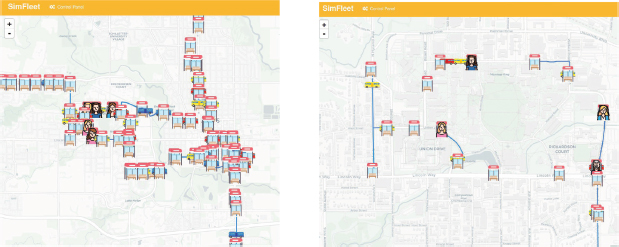
Figure 2. Visualisation of the public bus service of Ames through a SimFleet simulation
• Bus stop agents represent physical locations that enable the interaction between buses and customers. These agents keep an updated register of customers waiting at them and their desired destination. Once a bus halts at a specific bus stop, such a bus stop informs the waiting customers of the bus’ route. Customers that have a destination stop within the bus route board the vehicle, as long as the bus has enough capacity.
• Transport agents represent buses. Each bus travels through the stops of its route, following a predefined order. Once a bus reaches the end of its route, it begins traversing its stops again, either in the same (circular route) or reversed (linear route) order. Transport agents keep an updated list of their passengers and their destination stops. Each time a transport agent halts at a stop, a process is initiated for passengers to get off the bus. Then, customers waiting at the stop may board the vehicle, provided there is enough space for them.
• Customer agents represent the users of the bus service. Customers have a predefined origin and destination stop. They spawn at their origin bus stop and wait for the right bus to ride to their destination. In addition, as SimFleet allows for the dynamic introduction of agents in its simulations, each customer has a timestamp determining the time they spawn in the scenario. The set of all customers in the simulation conforms to the demand for the transportation service.
SimFleet’s simulation scenarios are configured in a JSON file containing information about the agents’ location, goals and spawn times. The outputs of the different ML models presented in Section 3 have been used to fill up a series of simulation configuration files that represent the Ames urban bus system. Specifically, one scenario per route is created, representing the bus service along it, between 6:00 (the first time at which passengers appear) and 23:30 (end of service).
The Google Maps API4 is employed to extract the exact location of each bus stop agent. The number of transport agents in each simulation is extracted from the dataset. Transport agents are initially deployed and uniformly distributed along the route. Their capacity is set to 60 passengers, which was the most common value in the data. Finally, the ML models are used to generate the demand shape in each simulation.
The number of passengers is determined using prediction through the obtained ML models. The passenger load is spatially and temporally distributed among stops and time periods using cross-distribution proportions calculated from historical onboarding data. The passenger offboarding, on the other hand, is determined with the Large Numbers Law (Erdös and Rényi, 1970), assigning a probability to each destination stop. The number of onboarding passengers assigned to each section and time period is predicted using the best model for each route.
Then, such a prediction is disaggregated to calculate the offboardings based on historical offboarding distribution data to assign probabilities for each stop. Therefore, passengers’ destinations are randomly selected based on these probabilities.
4.2. Route Performance Analysis
In this section, the performance of the urban bus fleet of Ames, Iowa, is assessed through several simulations that reproduce a typical service along some of its routes. The demand in each simulation, described by the number of users of the service and their origin/destination stops, is computed by the ML prediction models described in Section 3. Thus, one simulation per route is executed, and the results are subsequently analysed.
The performance of a transportation service is evaluated through the definition of specific metrics. During the simulation, agents gather data to quantify those metrics. With such a fine level of granularity, we could pinpoint underperforming agents and readjust the distribution of resources in the fleet. Nevertheless, given the high number of agents in the simulations and considering the scope of the paper, we combine individual agent metrics into a single global metric, presenting its average value and standard deviation. With this, global results are obtained that permit the assessment of fleet performance in each route. It must be noted, however, that the developed ML models allow for the creation of detailed scenarios, which may be used to compare fleet performance in a wide range of situations, such as specific days of the week or weather conditions.
Each simulation is characterised by its size in terms of number of agents. The performance metrics are divided into two groups: those indicating resource usage and those describing service quality. On the one hand, resource usage is shown by the distribution of passengers among the buses assigned to a route, referred to as ridership. A high standard deviation for the average ridership of the buses in a route indicates a poor distribution of the demand among the transports. In addition, if a bus has no passengers during the simulation, it is marked as an unused bus, generally indicating the route represented in the simulation has an excess of resources assigned to it. On the other hand, service quality metrics comprise the time needed by users, on average, to reach their destination. The portion of that time during which the user has been waiting at a bus stop is presented separately. Finally, we included the average distance driven by the buses assigned to a route as an extra metric of fleet performance in terms of fuel or energy consumption.
Table 5 presents the global results of all executed simulations. Simulations are identified by the route they represent and characterised by the amounts of stops, service users or pax, and buses. The number of unused buses is shown together with the average ridership in each bus, indicating the resource usage of the fleet. Then, average waiting and total times are presented, in minutes, giving a sense of the service quality along that route. Regarding resource usage, we observe that generally, the assigned number of transports is adequate for most routes. Routes 1 Red West and 5 Yellow break such a pattern by presenting 4 and 1 unused buses, respectively. The average ridership of the route’s buses, in terms of number of passengers, shows an interesting trend among all simulations. The standard deviation value is generally high, even surpassing the average for routes 1 Red West and 7 Purple, or matching it as in the cases of routes 1 Red West, 2 Green West and 14 Peach. The ridership of a bus is dependent on its position within the route at the times in which higher demand is present. As commented in Section 4.1, customer agents are temporally distributed in the simulation based on the ML models’ predictions. Because of that, such a distribution is a generalisation of the real-world observation; the data used to train the models. Transportation demand tends to present both peak periods in which a higher than usual number of users want to make use of the service, and low periods where very few potential customers are present. With that inmind, the trend in the average ridership values is to be expected, as the transportation demand is not uniformly distributed throughout the simulation. Ultimately, these results indicate that neither average nor individual values of bus ridership provide sufficient information to assess the allocation of buses to a route, as this value is closely dependent on the spatial and temporal relationship between transport and demand.
Table 5: Description and global metrics of each simulation (one per row). The first four columns identify the simulation and describe its size in terms of number of agents. Stops may be shared between different routes. Routes: (1E: 1 Red East, 1W: 1 Red West, 2E: 2 Green East, 2W: 2 Green West, 3: 3 Blue, 5: 5 Yellow, 7: 7 Purple, 9: 9 Plum, 11: 11 Cherry, 14: 14 Peach, 23: 23 Orange)
Route |
Stops |
Pax |
Buses (unused) |
Avg. ridership (num. of pax) |
Avg. waiting (min.) |
Avg. total (min.) |
Avg. distance (km) |
1E |
40 |
959 |
30 (0) |
32±31 |
2.2±1.9 |
21.3±12.8 |
222.7±0.4 |
1W |
42 |
890 |
31 (4) |
33±60 |
1.5±1.2 |
16.5±10.8 |
223.9±0.3 |
2E |
40 |
295 |
19 (0) |
16±10 |
2.3±2.1 |
20.6±10.0 |
239.3±0.5 |
2W |
40 |
261 |
18 (0) |
15±14 |
2.9±2.3 |
19.9±12.5 |
288.7±0.4 |
3 |
32 |
2122 |
20 (0) |
106±80 |
2.9±3.0 |
13.5±8.9 |
226.1±0.3 |
5 |
21 |
23 |
5 (1) |
6±2 |
4.9±3.3 |
17.9±9.3 |
187.2±0.2 |
7 |
20 |
324 |
6 (0) |
54±74 |
4.2±2.9 |
14.0±4.9 |
174.0±0.1 |
9 |
30 |
634 |
10 (0) |
64±46 |
5.0±4.8 |
15.4±10.5 |
270.8±1.0 |
11 |
31 |
1530 |
18 (0) |
85±64 |
2.6±2.0 |
15.2±7.9 |
228.5±0.3 |
14 |
33 |
45 |
5 (0) |
9±9 |
7.1±4.4 |
24.8±10.2 |
181.7±0.5 |
23 |
16 |
4300 |
33 (0) |
130±81 |
1.4±1.5 |
13.7±6.7 |
164.9±2.0 |
Furthermore, in terms of service quality, results show a generally acceptable user waiting time in all routes, ranging between 2 and 7 minutes. Route 1 Red West stands out as the route with the lowest waiting time at an average of 1.5 minutes. As commented above, this route also presents 4 unused buses. This points to the fact that the route has a number of buses allocated to it that do not match their predicted demand. Route 14 Peach presents the highest waiting times, on average. This route, however, presents low demand and number of buses, probably causing longer waiting periods. Route 9 Plum stands out as the middle-sized scenario (634 users and 10 buses) with the highest average waits, being around 5 minutes. The average total time values vary in a higher range than the waiting times, as the former is more related to the route’s length and its number of stops. This metric presents a higher standard deviation, which is to be expected as different combinations of origin/destination stops greatly affect a passenger’s trip. Finally, the distance travelled by the different buses of a route is very close, as the low standard deviation values reflect.
4.3. Effect of Fleet Configuration
The experimentation of Section 4.2 illustrates how ML prediction and multi-agent simulation can be combined to evaluate the performance of a transportation service. The flexibility of simulations, however, permits the tuning of the reproduced system through many iterations of changing its configuration, running the new simulation, and analysing the results. In this section, we focus our interest on three routes of the Ames urban bus system that showed some particularities in the performance assessment results. With the following experimentation, we intend to exemplify how the proposed system can be used to advise on the configuration of transportation services adapted to their expected demand.
The routes selected for further experimentation are 1 Red West, 3 Blue and 9 Plum. Firstly, route 1 Red West presents 4 unused buses and a very uneven distribution of passengers. Secondly, route 3 Blue presents the second highest demand in any route. Finally, route 9 Plum presents the highest waiting time for middle-sized simulations (in terms of the number of agents), as commented before. Moreover, we explore the global effects of bus fleet variation on resource usage and service quality at these routes.
Table 6 presents the most relevant configurations from all the varying configurations tested for the aforementioned routes. Simulations are identified by the route they reproduce and the number of transports that were added or subtracted from the baseline fleet. The number of transports varied in intervals of 5 buses for routes 1 Red West and 3 Blue, whereas route 9 Plum had smaller variations, as its original number of transports was only 10. The results of new configurations are presented next to the baseline configuration results, which are highlighted in italics. A global assessment of the results points towards the expected correlation between the number of buses servicing a route and lower waiting times. In terms of ridership, we observe the same trend as in Section 4.2. The mere addition or subtraction of transports to the fleet does not have a proportional effect on the average ridership values. If those values were to be improved, achieving a more uniform distribution of passengers among buses, the simulation should be analysed on a finer level, taking into account the temporal and physical distribution of the demand peaks.
Table 6: Global metrics of each simulation (one per row). Simulations are identified by the route they reproduce and the number of transports that were added or subtracted from the baseline fleet. The baseline simulation results are indicated in italics. The layout of stops and the demand of each route have been preserved as in the baseline simulation. The number of buses in each route varies along its simulations. Routes: (1W: 1 Red West, 3: 3 Blue, 9: 9 Plum).
Route |
Buses (unused) |
Avg. assignments (num. of pax) |
Avg. waiting (min.) |
Avg. total (min.) |
Avg. distance (km) |
1W |
31 (4) |
33±60 |
1.5±1.2 |
16.5±10.8 |
223.9±0.3 |
1W-5 |
26 (3) |
39±60 |
2.1±1.6 |
17.3±10.5 |
223.1±0.4 |
1W-10 |
21 (1) |
45±62 |
2.2±1.6 |
17.4±10.7 |
223.8±0.4 |
1W-15 |
16 (0) |
56±80 |
2.5±1.7 |
17.7±10.5 |
223.0±0.5 |
1W-20 |
11 (0) |
81±100 |
5.4±4.1 |
20.7±10.8 |
224.0±0.6 |
|
|||||
3+15 |
35 (0) |
62±49 |
2.6±2.8 |
13.3±8.8 |
226.1±0.3 |
3+10 |
30 (0) |
71±56 |
3.1±3.5 |
13.8±9.0 |
226.0±0.4 |
3+5 |
25 (0) |
85±70 |
3.1±3.1 |
13.8±8.9 |
226.5±0.3 |
3 |
20 (0) |
106±80 |
2.9±3.0 |
13.5±8.9 |
226.1±0.3 |
3-5 |
15 (0) |
142±98 |
4.6±4.2 |
15.4±9.2 |
226.2±0.6 |
3-10 |
10 (0) |
212±113 |
6.7±5.8 |
17.5±9.9 |
225.5±0.8 |
3-15 |
5 (0) |
425±288 |
8.2±5.5 |
19.2±9.8 |
225.7±1.5 |
|
|||||
9+5 |
15 (0) |
42±37 |
2.7±2.3 |
13.2±9.3 |
271.0±0.9 |
9+3 |
13 (0) |
49±40 |
4.4±4.7 |
14.9±10.5 |
270.6±0.8 |
9+1 |
11 (0) |
58±38 |
4.7±4.9 |
15.1±10.5 |
271.1±0.9 |
9 |
10 (0) |
64±46 |
5.0±4.8 |
15.4±10.5 |
270.8±1.0 |
9-1 |
9 (0) |
71±40 |
5.1±4.4 |
15.5±10.5 |
270.9±1.0 |
9-3 |
7 (0) |
91±74 |
5.7±4.9 |
16.2±10.4 |
271.5±1.0 |
9-5 |
5 (0) |
127±62 |
6.8±5.0 |
17.3±10.6 |
271.6±0.9 |
Analysing the specific results of each route, it can be observed how, for route 1 Red West, a reduction in the number of buses does not immediately cause the expected disappearance of unused buses. In fact, 15 buses had to be subtracted from the fleet to achieve the first result with no unused buses. Moreover, the average waiting times do not severely worsen until 20 buses have been removed from the original fleet. These results show the general complexity of the dynamics of transportation systems. In particular, route 1 Red West seems to present particularities in its predicted demand that again warrant more detailed analysis to determine which of its buses are not performing adequately.
Results for route 3 Blue show how a higher volume of demand causes a higher variation in the service quality metrics. The average waiting times in route 3 Blue simulations increase at greater steps with the reduction of the fleets than in other simulations. Similarly to what we observed in route 1 Red West, however, the mere increase of fleet vehicles does not cause a proportional reduction of the average user waiting time, as the simulations with 5 and 10 extra transports reflect. This is likely caused due to the particularities of the predicted demand for that route, whose shape may cause the waiting times to stay the same for specific time periods even if more buses were added, thus affecting the global average.
Finally, route 9 Plum presents relatively uniform results with respect to the service quality, whose times increase and decrease relatively proportional to the excess or lack of buses. The average ridership presents the same behaviour, although its standard deviation is not reduced or augmented proportionally to the fleet vehicles, thus indicating, again, that a more even allocation of passengers is not achieved.
5. Discussion
Along Section 4, we have proved the utility of ML techniques together with agent-based simulation to assess the performance of transportation fleets. For this work, the experimentation was developed using data from the urban bus service of Ames, Iowa. Such a service was simulated to illustrate the use of our proposal. The results analysed in Sections 4.2 and 4.3 bring key insights into the global operation of the service in each of its routes. It is important, however, to contextualise the results and their scope, discussing the limitations of the used approaches.
The demand data in the simulations was generated by a series of ML prediction models, each developed specifically for a route. As explained in Section 2, the approach of an individual model per route was chosen given the inconsistencies in the available data. In addition, the transformations applied to the data before training the models have an evident effect on the model’s final outputs. Ideally, a single model considering all the dataset information would have been developed, leading to a better scenario for global performance assessments. As that was not the case, our global assessments are individual for each route and not the whole urban bus system. The biases of the ML models must be taken into account as they were used to generate the demand data for our simulations.
Agent simulation is a great tool to test modifications on real-world systems without actually implementing those changes. For the case of transportation services, this is especially relevant, as changes in their configuration have a considerable impact. Nevertheless, the exact reproduction of a transportation system is hard to achieve, as
they generally have many involved actors and a high level of dynamism. Our simulation scenarios realistically represent the routes of Ames bus service geographically. However, the metrics chosen to evaluate simulations have been defined by us. The value of such metrics, in turn, is determined by the simulation execution and is therefore vulnerable to noise.
The above discussion evidences that one must be careful when drawing conclusions from the simulation results. In our experimentation for this work, we must highlight that demand data was predicted by ML models, which, even though they accurately generalise the training data, may not be a close enough reproduction of the complexity and detail of real demand dynamics. Because of that, our results and their subsequent assessment should not be understood as direct recommendations for the improvement of the service. Nevertheless, a lack of precision does not imply a lack of usefulness. The analysis of a simulation does reveal possible paths for a potential improvement of many aspects of the reproduced system. Our results expose trends regarding the ridership distribution and service quality in each route. Therefore, the proposed system could be used to help transportation operators make more informed decisions about the configuration of their services and even decide more specific directions of future research.
6. Conclusions
The improvement of transportation services poses unique challenges, as it involves complex dynamics among many moving parties. In this work, passenger flow prediction models have been developed to guide the enhancement of urban bus-based transportation systems. Data from the urban bus service of Ames, Iowa, has been employed to train several ML prediction models. Before the training, the data was analysed, cleaned, and combined with historical precipitation and snow depth data to bring a more realistic perspective to the models’ predictions. Our approach to transportation improvement was completed through agent-based simulation. Specifically, the models were used to develop various scenarios, which, executed in SimFleet, allowed for the assessment of the global performance of Ames’ bus service in each of its routes. The results of our various experiments illustrate the combined use of prediction models and simulation to analyse the performance of a transportation system and test modifications on its operation.
The presented approach aims to aid transportation service operators in their decision-making when it comes to the configuration of their systems. The simulations’ results can be assessed within their context to reveal specific trends and problems derived from aspects of the service, such as its resource allocation or service quality. In addition, the present global analysis of results is useful to discover and select more detailed paths of research for future transportation optimisation efforts.
In terms of contributing to machine learning applications, the current work is our first approach to realistic transportation demand generation based on forecasts. This line of research will continue with the intention of improving both the prediction models and the subsequent validation through simulation. The simulation scenarios developed for this paper fit the scope of illustrating the usefulness of the proposal but lack the necessary detail to extract specific instructions and improve a service such as the Ames urban bus. The developed ML predictors have the potential to predict demand data for far more specific scenarios than the ones analysed, thus being useful in reproducing demand patterns on different days of the week, different months, and even rainy or snowy weather. For future research, more detailed simulation scenarios will be set up and addressed. In addition, we are currently working on the creation of models for resource prediction, which would guide the creation of a transport fleet that better matches the requirements of each route.
Finally, regarding the simulations’ development, there have been limitations concerning the distribution of buses and their movement between stops on their routes. In future work, aspects such as the number of active buses per time period will be established, and, in addition, a more flexible movement of these buses within their assigned route will be allowed. We have a particular interest in demand-responsive mobility and the improvement its application could bring to those lines with lower demand.
7. Funding
This work is partially supported by grants PID2021-123673 and PDC2022-133161-C32 funded by MCIN/AEI/ 10.13039/501100011033 and by «ERDF A way of making Europe». Pasqual Martí is supported by grant ACIF/2021/259 funded by the «Conselleria de Innovación, Universidades, Ciencia y Sociedad Digital de la Generalitat Valenciana». Jaume Jordán is supported by grant IJC2020-045683-I funded by MCIN/AEI/ 10.13039/501100011033 and by «European Union NextGenerationEU/PRTR».
References
AlKhereibi, A. H., Wakjira, T. G., Kucukvar, M., and Onat, N. C., 2023. Predictive Machine Learning Algorithms for Metro Ridership Based on Urban Land Use Policies in Support of Transit-Oriented Development. Sustainability, 15(2). ISSN 2071-1050. https://doi.org/10.3390/su15021718.
Baghbani, A., Bouguila, N., and Patterson, Z., 2023. Short-Term Passenger Flow Prediction Using a Bus Network Graph Convolutional Long Short-Term Memory Neural Network Model. Transportation Research Record, pages 1331–1340.
Bishop, C., 1995. Neural networks for pattern recognition. In Oxford university press.
Breiman, L., 2001. Random Forests. Machine Learning, Vol 45:5–32.
Cortes, C. and Vapnik, V., 1995. Support-vector networks. Machine Learning, 20:273–297.
Drucker, H., Burges, C. J., Kaufman, L., Smola, A., and Vapnik, V., 1996. Support vector regression machines. Advances in neural information processing systems, 9.
Elman, J. L., 1990. Finding structure in time. Cognitive science, 14(2):179–211.
Erdös, P. and Rényi, A., 1970. On a new law of large numbers. Journal d’Analyse Mathématique, 22:103–111.
Gers, F. A., Schmidhuber, J., and Cummins, F., 2000. Learning to forget: Continual prediction with LSTM. Neural computation, 12(10):2451–2471.
Goodfellow, I., Bengio, Y., and Courville, A., 2016. Deep learning. MIT press.
Gunawan, F., Suharjito, S., and Gunawan, A., 2014. Simulation Model of Bus Rapid Transit. EPJ Web of Conferences, 68.
Hajinasab, B., Davidsson, P., Persson, J., and Holmgren, J., 2016. Towards an Agent-Based Model of Passenger Transportation. pages 132–145.
Haykin, S., 2009. Neural networks and learning machines, 3/E. Pearson Education India.
He, M., Muaz, U., Jiang, H., Lei, Z., Chen, X., Ukkusuri, S. V., and Sobolevsky, S., 2022. Ridership prediction and anomaly detection in transportation hubs: an application to New York City. The European Physical Journal Special Topics, 231(9):1655–1671.
Ibáñez, A., Jordán, J., and Julian, V., 2023. Improving Public Transportation Efficiency Through Accurate Bus Passenger Demand. In Durães, D., González-Briones, A., Lujak, M., El Bolock, A., and Carneiro, J., editors, Highlights in Practical Applications of Agents, Multi-Agent Systems, and Cognitive Mimetics. The PAAMS Collection, pages 18–29. Springer Nature Switzerland, Cham. ISBN 978-3-031-37593-4.
Julong, D. et al., 1989. Introduction to grey system theory. The Journal of grey system, 1(1):1–24.
Liaw, A., Wiener, M. et al., 2002. Classification and regression by randomForest. R news, 2(3):18–22.
Liu, S. and Forrest, J. Y. L., 2010. Grey systems: theory and applications. Springer Science & Business Media.
Liu, Y., Liu, Z., and Jia, R., 2019. DeepPF: A deep learning based architecture for metro passenger flow prediction. Transportation Research Part C: Emerging Technologies, 101:18–34.
Liyanage, S., Abduljabbar, R., Dia, H., and Tsai, P., 2022. AI-based neural network models for bus passenger demand forecasting using smart card data. Journal of Urban Management, 11:365–380.
Lv, L., Hu, D., and Liu, X., 2024. An EEMD-EWT-LSTM-based short-term prediction approach for inbound metro ridership. Journal of Industrial and Management Optimization. ISSN 1547-5816. https://doi.org/10.3934/jimo.2024035.
Ming, W., Bao, Y., Hu, Z., and Xiong, T., 2014. Multistep-Ahead Air Passengers Traffic Prediction with Hybrid ARIMA-SVMs Models. The Scientific World Journal, 2014.
Nagaraj, N., Gururaj, H., Swathi, B., and Hu, Y., 2022. Passenger flow prediction in bus transportation system using deep learning. Multimed Tools Appl, 81:12519–12542.
Nair, G. S., Mirzaei, A., and Ruiz-Juri, N., 2023. Investigating the Use of Machine Learning Methods in Direct Ridership Models for Bus Transit. Transportation Research Record, 2677(3):768–781. https://doi.org/10.1177/03611981221117540.
Palanca, J., Terrasa, A., Carrascosa, C., and Julián, V., 2019. SimFleet: A New Transport Fleet Simulator Based on MAS. In Highlights of Practical Applications of Survivable Agents and Multi-Agent Systems. PAAMS Collection, pages 257–264. Springer.
Santanam, T., Trasatti, A., Hentenryck, P. V., and Zhang, H., 2024. Public Transit for Special Events: Ridership Prediction and Train Scheduling. IEEE Transactions on Intelligent Transportation Systems, pages 1–17. https://doi.org/10.1109/TITS.2024.3373634.
Schmidhuber, J. and Hochreiter, S., 1997. Long Short-Term Memory. Neural Computation, 9:1735–1780.
Vapnik, V., 2013. The nature of statistical learning theory. Springer science & business media.
Wang, X., Guo, Y., Bai, C., Liu, S., Liu, S., and Han, J., 2020. The Effects of Weather on Passenger Flow of Urban Rail Transit. Civil Engineering Journal, Vol 6, No 1:11–20.
Wilbur, K., 2022. CyRide Automatic Passenger Counter Data, 10/2021-06/2022.
Zhang, Z., Xu, X., and Wang, Z., 2017. Application of grey prediction model to short-time passenger flow forecast. AIP Conference Proceedings, 1839.
_______________________________
1 https://www.statista.com/chart/25129/gcs-hoW-the-world-commutes/.Model
2 https://www.event.iastate.edu/?sy=2023&sm=01&sd=26&featured=1&s=d