ADCAIJ: Advances in Distributed Computing and Artificial Intelligence Journal
Regular Issue, Vol. 14 (2025), e31737
eISSN: 2255-2863
DOI: https://doi.org/10.14201/adcaij.31737
Machine Learning Based Prediction of Retinopathy Diseases Using Segmented Retinal Images
Sushil Kumar Saroja, Rakesh Kumara, and Nagendra Pratap Singhb
a Computer Science and Engineering Department, MMM University of Technology, India, 273010
b Computer Science and Engineering Department, NIT, Jalandhar, India, 144011 sushil.mnnit10@gmail.com, rkcs@mmmut.ac.in, singhnp@nitj.ac.in
ABSTRACT
Diabetes, hypertension, obesity, glaucoma, etc. are severe and common retinopathy diseases today. Early age detection and diagnosis of these diseases can save human beings from many life threats. The retina’s blood vessels carry details of retinopathy diseases. Therefore, feature extraction from blood vessels is essential to classify these diseases. A segmented retinal image is only a vascular tree of blood vessels. Feature extraction is easy and efficient from segmented images. Today, there are existing different approaches in this field that use RGB images only to classify these diseases due to which their performance is relatively low. In the work, we have proposed a model based on machine learning that uses segmented retinal images generated by different efficient methods to classify diabetic retinopathy, glaucoma, and multi-class diseases. We have carried out extensive experiments on numerous images of DRIVE, HRF, STARE, and RIM-ONE DL datasets. The highest accuracy of the proposed approach is 90.90 %, 95.00 %, and 92.90 % for diabetic retinopathy, glaucoma, and multi-class diseases, respectively, which the model detected better than most of the methods in this field.
KEYWORDS
segmented images; machine learning; feature extraction; disease classification
1. Introduction
Diseases have long posed a profound threat to life and biodiversity. Several life-threatening retinopathy diseases are obesity, diabetes, macular degeneration, hypertension, arteriosclerosis, glaucoma, etc. World Health Organization (WHO) published a report that 2.2 billion population in the world are suffering from vision impairment. Around 1.28 billion population between the 30-79 age group have hypertension. By 2019, there were about 463 million people between the ages of 20 and 79 who had diabetes. By 2016, there were around 650 million obese adults worldwide. The blood vessels of the retina withhold details regarding these life-threatening diseases. For instance, the shape, structure, or color of a retinal vessel alters in response to conditions such as diabetes, hypertension, etc. The ratio of the optic cup to the disc is increased in glaucoma cases. Figure 1 depicts a glaucoma disease infected retina image. Medical professionals believe that these serious illnesses can be cured with early detection, prompt diagnosis, and appropriate medication follow-up. Hence, it is necessary to extract features from vessels and predict these diseases.
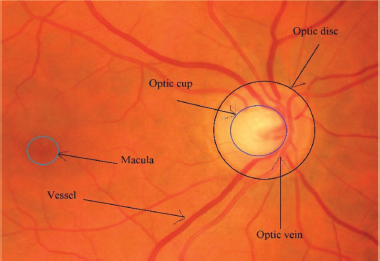
Figure 1. A glaucoma disease infected fundus image of the retina
A traditional approach (hand operated procedure) of feature extraction and classification is time consuming, prone to mistakes, and needs extensive training. Meanwhile, a software based approach is simpler, more efficient, and less expensive. There are various automatic classification methods today such as machine learning and deep learning based methods. Deep learning based methods require a lot of processing power and time, and many input images compared to machine learning methods. Existing automatic methods for retinal disease classification have worked on RGB images of the retina. However, the effect of diseases reflects mostly on retinal blood vessels and optic discs. A segmented image is a vascular tree of vessels and focuses only on the object while an RGB image may contain additional background and unrelated objects that could mislead the classifier. A segmented image has generally good contrast which makes distinguishing features more prominent. This image effectively helps the model learn more distinct and meaningful features, resulting in better performance. The proposed model is based on machine learning that uses segmented retinal images. The model has better accuracy compared to the present models in this field. The paper’s main contributions are:
•A rigorous analysis of different feature extraction and classification techniques.
•The design of an approach based on segmented images for retinal disease classification.
•Presented detailed results that are obtained by conducting in-depth experiments on numerous images.
The paper’s subsequent sections are arranged as: Section 2 explores the most recent methods for classifying retinal diseases. A model for improved feature extraction and retinal disease classification has been described in Section 3. The results and analysis of the model are presented in Section 4. Finally, the paper concludes with future research in Section 5.
2. Related Work
The blood vessels of a retina carry details that point to various severe retinopathy diseases. This attracted researchers and academicians to propose models for retinal disease prediction and feature extraction. Various prominent models for retinal disease prediction and feature extraction are explored (Attia et al., 2020; Muchuchuti et al., 2023; Sengar et al., 2023; Alam et al., 2023). Some of them are discussed below:
Zhu et al. (2022) proposed six-category deep learning methods that employed the ResNet50 and EfficientNet-B4 for retinal disease classification. They classified five different retinal diseases i.e., retinal vein occlusion (RVO), high myopia, glaucoma, diabetic retinopathy (DR), and macular degeneration. They took 400 retinal images for each type of disease. Additionally, they took 400 healthy retinal images. Therefore, in total, they took 2400 RGB retinal images for classification. The method used 2400 images of the retina for training and 1315 for the testing process. Pin et al. (2022) proposed a transfer learning based model for the prediction of retinal diseases. They used quality evaluation first in the prediction system to remove poor-quality images. Second, the transfer learning method was applied with different convolutional neural network (CNN) methods to predict glaucoma, macular degeneration, and diabetic retinopathy diseases. The authors used 1340 RGB retinal images in the method.
Abitbol et al. (2022) developed a deep learning based method to find sickle cell retinopathy, DR, and RVO. They applied DenseNet121 model of CNN to classify retinal diseases. The effectiveness of the approach was evaluated using the k-fold cross-validation. An established augmentation method was used to increase the accuracy of the approach. They utilized 224 ultra wide field color fundus photography retinal images where there were 169 vascular diseases and 55 healthy images. Cao et al. (2022) designed an attentional system and improved ResNet based method for the classification of diabetic retinopathy diseases. The authors modified the design of residual blocks and improved the down-sampling level to increase the information about a feature at the hidden layer. Moreover, an attention system was used to increase the extraction of features. The authors took 35126 RGB retinal images. They increased the number of images up to 40000 by the data augmentation technique. They used 35000 RGB retinal images for training and 5000 for testing processes.
Shrivastava et al. (2021) have given an approach to classify DR and macular degeneration retinal diseases. In the approach, the authors applied CLAHE to crop and enhance retinal images. They also applied data augmentation operations i.e., rotation, vertical and horizontal flip in the approach. The authors used Efficient-Net B4 and B7 models of CNN to classify the various retinal diseases. The authors used 3264 RGB retinal images to train and 427 images to test the model. Londhe et al. (2021) designed a model to classify various retinal diseases i.e., glaucoma, diabetes, cataract, and other retinal diseases. The authors used InceptionV3, DenseNet169, transfer learning, and InceptionResNetV2 techniques in the model to extract the retinal features. They used the LSTM method to identify diseases from extracted features. The authors used 1200 RGB images of the retina to evaluate the proposed model. The accuracy of the model is relatively low.
Virmani et al. (2019) designed a model for the classification of retinopathy diseases. In the model, a contrast stretching operation was performed. The authors extracted the Gray level co-occurrence matrix, first order statistics, and gray-level run length matrix features in the method. They used the probabilistic artificial neural network to classify DR and glaucoma diseases. The method is tested on very few images that is the 45 RGB images of HRF where 15 showed glaucoma, 15 showed diabetic retinopathy, and 15 showed healthy images. The authors have trained their proposed model on 8 images and tested it on 7 images only for each category. The method was tested on a single data set and a smaller number of images. Their model has achieved the highest accuracy of 85.71 % corresponding to extracted gray-level run length matrix features.
Sarki et al. (2020) proposed a model for retinal disease classification. In the model, the authors used convolutional neural network models on ImageNet. The authors also used different performance improvement methods such as fine-tuning, contrast enhancement, and optimization. The methods classify the mild and moderate multi class DR diseases. The authors used 3149 RGB retinal images of various datasets i.e. the DRISHTI-GS, Messidor-2, Messidor, and Cataract retinal. Han et al. (2021) developed a generative adversarial network (GAN) based anomaly detection model for the classification of glaucoma, myopia, diabetic retinopathy, cataract, macular degeneration, and hypertensive retinopathy diseases. In the pre-processing phase, low quality images were discarded manually. They used 90499 RGB retinal images in the approach. There were 64351 normal and 26148 unhealthy images. The accuracy of the method was not very good.
Das et al. (2019) designed a framework for retinopathy disease identification. In the framework, a transfer learning technique is used to classify glaucoma, healthy, and diabetic retinopathy diseases. In the preprocessing phase, an augmentation operation was conducted to increase numerous retinal images. The data augmentation technique includes flipping, rotation, and cropping of images. The method was tested on RGB retinal images which consisted of glaucoma, healthy, and diabetic diseases. The approach was tested on a single dataset. Nazir et al. (2021) proposed an approach to predict diabetic macular edema and diabetes retinal diseases. In the approach, the authors used the DenseNet-100 deep learning method to extract the retinal features. The CenterNet method was applied to classify the diseases. They used 4178 RGB images of the retina from APTOS 2019, and IDRiD datasets. They used EYEPACS and Diaretdb1 datasets to carry out the cross dataset validation. From the above discussion, we found that the existing methods for retinal disease classification have been tested on RGB images of the retina. Most of the methods are deep learning methods.
3. Proposed Approach
The proposed model is a machine learning based model that works on the segmented images of the retina. In the model, we first extract various features from segmented images using different feature extraction techniques. After that, we classify the retinal diseases based on these extracted features using different machine learning classifiers. Figure 2 depicts the image processing phases of the proposed model.
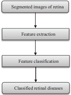
Figure 2. Flow diagram of the proposed model
3.1. Segmentation Methods
We have used segmented images generated by the Gaussian match filter, Fréchet match filter, Wald match filter, and a deep learning method (UNET). Retinal images generally have poor contrast due to which it is difficult to find a clear vascular tree of blood vessels. Although the effect of disease reflects mostly on retinal blood vessels, the match filter increases the contrast of retinal images due to which the obtained segmented images have clear vascular trees of blood vessels. The segmentation process has three major phases. Pre-processing phase: In this phase Principal component analysis (PCA), Contrast-limited adaptive histogram equalization (CLAHE), or multi-scale switching morphological operator (MSMO) method is used to enhance the retinal images. Match filter phase: In this phase, we have used the Gaussian, Fréchet, or Wald match filter to increase the contrast of retinal images. Post-processing phase: In this phase, we have used the optimal or Otsu thresholding method to get a vascular tree of blood vessels of a retinal image. Also, we have used length filtering and masking operations to get a clear vascular tree of vessels.
Fréchet probability distributions function (PDF) is an extremely valued PDF. Wald PDF is a two-parameter family of continuous probability distributions with support on (0, ∞). These PDFs have skewed characteristics. Fréchet and Wald PDF based match filters are two new match filters for vessel segmentation. Gaussian PDF is a continuous distribution function. It has symmetric characteristics. Modified Gaussian is the inverse of Gaussian. Modified Gaussian PDF based match filter is a new match filter. UNET architecture is an end-to-end trainable model. It is a fully CNN-based model that comprises two parts, similar to auto-encoder models. Each block is made of two convolutional layers that are followed by a ReLU function and a polling layer. The performance of these segmented methods is depicted in Table 1. Figure 3 shows the fundus RGB image of the 1_test.tif image of the DRIVE. Figure 4 shows the segmented image of 1_test.tif.
Table 1. Performance of used segmentation methods
Methods |
Recall |
Specificity |
Accuracy |
Fréchet match filter based method |
0.7307 |
0.9761 |
0.9544 |
Wald match filter based method |
0.7217 |
0.9880 |
0.9558 |
Modified Gaussian match filter based method |
0.6747 |
0.9850 |
0.9577 |
Deep learning (UNET) method |
0.8060 |
0.9750 |
0.9560 |
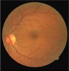
Figure 3. RGB image of 1_test.tif image
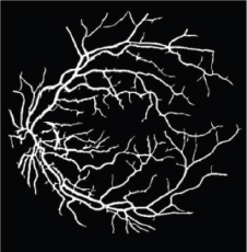
Figure 4. Segmented image of 1_test.tif image
3.2. Feature Extraction Methods
We have used gray-level co-occurrence matrix (GLCM), Laws texture energy (LTE), Tamura, wavelet, local binary pattern (LBP), and histogram of oriented gradients (HOG) methods for feature extraction from segmented retinal images. GLCM contains rich texture patterns, particularly in regions like optic discs, blood vessels, and pathological areas. It is robust to noise and illumination changes which are common challenges in retinal imaging. In turn, LTE focuses on capturing low-energy textures, which helps in detecting fine and smooth textures that are common in retinal images. Like GLCM, it is also less sensitive to noise and illumination change. Meanwhile, Tamura effectively captures both global and local texture characteristics. In retinal images, this is crucial for distinguishing between healthy and diseased regions. On the other hand, Wavelets can decompose the image into multiple scales and resolutions, enabling the capture of both fine details and broader structures of the retina. In turn, LBP excels at capturing micro-textures which are essential in retinal images for identifying fine details. Retinal images often suffer from uneven illumination. LBP is robust to changes in lighting conditions ensuring that the extracted texture features remain consistent even under varying image qualities. Lastly, HOG emphasizes edge orientation and gradient distribution, making it robust to variations in lighting and minor deformations.
3.2.1. Gray Level Co-Occurrence Matrix
It is a statistical approach to mining the texture of an image (Haralick et al., 1973). Pixel spatial relationships are taken into account as a GLCM matrix. It calculates the frequency for sets of pixels with particular values that happen in an image to classify texture. The GLCM matrix is first generated, and then statistical texture metrics are computed based on the matrix. Some of them are contrast, energy, homogeneity, entropy, dissimilarity, etc. These are defined as follows:
where n refers to the gray level numbers, while A(a,b) is the grayscale’s normalized value at kernel positions a and b, with a sum of 1.
3.2.2. Law’s Texture Energy
It is a method that applies local masks to identify different types of texture features (Laws et al., 1980). It designs a texture-energy mechanism that determines the number of variations within a fixed size window. The convolution mask size is 5 x 5. A collection of these nine masks is used to compute texture energy. Local masks were generated from the vectors E5, L5, S5, R5. The 5, L5, S5, and R5 vectors correspond to edge, level, spot, and ripple, respectively. Edge, level, spot, and ripple are the four main characteristics of the image. Let each of the resulting filtered images be denoted. gk for k ∊{E5, L5, S5, R5}2. From them, we can construct the texture energy images hk by computing the sum of the absolute intensities of the respective feature images in a (2P+1) × (2Q+1) neighborhood.
3.2.3. Tamura
It is based on psychophysical research on the six fundamental factors related to human visual perception (Tamura et al., 1978). These six fundamentals are line likeness, coarseness, regularity, contrast, roughness, and directionality. Coarseness, contrast, and directionality fundamentals are related to human perception more than the other three. For these reasons, we have considered only coarseness, contrast, and directionality features in the proposed work. These are defined as follows:
Coarseness: First computes the average corresponding to a neighborhood of 2k x 2k at coordinates (x, y) as follows:
Thereafter, for each point, the differences between pairs of averages are computed as follows:
Then for every single point, we select k that maximizes E in any direction. The coarseness measure is the average of Sopt(x,y)=2kopt over the image.
Contrast: It is defined mathematically as follows:.
where , α standard deviation, σ2 variance, and μ moment about the mean.
Directionality: For each peak i in a histogram with several peaks n, let φi be the angular position of the peak in ωi and ωi be the window of bins from the preceding valley to the subsequent valley. Let r be the normalization factor and (φ) be the height of a bin at angular point φ. The directionality (fdir) from the sharpness of HD is computed as follows:
3.2.4. Wavelet Transform
It breaks a function into a group of wavelets (Mallat et al., 1989). Wavelets possess two fundamental characteristics: location and scale. A wavelet’s «stretched» or «squished» state is determined by its scale. The wavelet’s location indicates its place in space or time. The fundamental idea behind wavelets is to analyze signals according to scale. Continuous, and discrete are the two wavelet transforms. These are described as follows:
where T is a real signal, ψ is an arbitrary mother wavelet, a is scale, b is location, and t is the time parameter.
where T is a real signal, ψ is an arbitrary mother wavelet, m is scale, n is translation, and t is the time.
3.2.5. Local Binary Pattern
It is a technique that is applied to find the texture features of surfaces (Ojala et al., 2002). In this method, the probability of texture pattern is summarized in a histogram. The formal expression of the LBP is stated as:
where P is the neighborhood pixels, ni refers to the ith neighboring pixel, and c refers to the center pixel. The histogram property of size 2P are segmented from the generated LBP code.
3.2.6. Histogram of Oriented Gradients
This method totals incidents of gradient orientation in localized portions of an image (Korkmaz et al., 2017), (Qin et al., 2016). It focuses on the shape or structure of an object. It utilizes the angle and magnitude of the gradient to calculate features. It produces histograms by applying the magnitude and orientations of the gradient for image regions. Assume a block of 3 x 3 pixels. Gradients for each pixel are computed as:
where dp and dq are horizontal and vertical gradients respectively, I(p, q) is pixel value at coordinate (p, q). The gradient (θ) is represented as:
3.3. Classification Methods
The proposed approach has applied machine learning methods on segmented retinal images for retinal disease classification. If images are segmented, machine learning (ML) methods efficiently use hand-crafted features (such as texture, shape, etc.) from segmented regions. Hand-crafted features capture disease characteristics well. These methods can automatically handle categorical features and exploit feature interactions without as much pre-processing. ML methods can outperform deep learning in disease classification using segmented images when a dataset is noisy, small, imbalanced, and lacks diversity.
3.3.1. Support Vector Machine
It aligns new instances to one of the classes by defining a separable hyperplane (Cortes et al., 1995; Boser et al., 1992). It finds first the ‘maximum-margin’ hyperplane. The maximum-margin hyperplane helps in finding the separation of points having a class with 1 from a class with 0 as depicted in Figure 5. Support vectors are the points that are closest to the hyperplane. Hyperplane h(x) is stated as:
where b is the fixed value of the distance from the origin, ω is a coefficient vector, and x is a specimen point. If h(x)>=0 in the linear SVM example, the points will be in class 1; otherwise, they will be in class 0. The following is the definition of the maximum distance (d) between the two distinct support vectors:
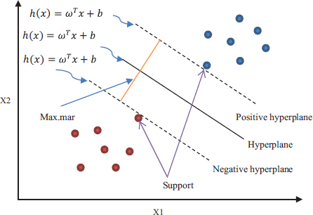
Figure 5. Support vector machine classifier
3.3.2. Logistic Regression
It is a predictive analysis approach based on the concept of probability (Tolles et al., 2016). It classifies the dependent variable that is categorical by using a given collection of independent variables. Its hypothesis expectation is described as:
The logistic regression cost function is stated as:
The logistic regression hypothesis is defined as:
3.3.3. K-Nearest Neighbor Methods
It is a supervised, and lazy method that is used in classification (Fix et al., 1951; Cover et al., 1967). It stores all the possible cases while training and classifies new observations by the value of its k-nearest neighbors’ majority. In the testing process, new observation is classified by calculating the similarity metric. One crucial element of the k-nearest neighbor (KNN) algorithm is the choice of value ‘k’ as it will determine how well the data can be utilized to generalize the result. In KNN, the similarity metric is the distance. Smaller distance refers to a more similar feature. In KNN, generally, Euclidian distance is considered in the classification process. Assuming that x and y represent the values on the x and y axes, respectively, then Euclidean distance (Ed) is defined as follows:
3.3.4. Discriminant Analysis
It is a classification method. Logistic regression is a classification algorithm traditionally limited to only two class prediction problems (Fisher et al., 1936; McLachlan et al., 2004). If you have more than two classes, then LDA is preferred.
where P is projection, Sb is between-class variance, and Sw is within-class variance. Quadratic Discriminant Analysis (QDA) is a variant of LDA. In QDA, each class uses its estimate of variance.
3.3.5. Ensemble Classifier
In this classifier, different base classifiers are generated which results in a new classifier that outperforms all constituent classifiers (Opitz et al., 1999; Rokach et al., 2010). The training set, representation, hyperparameters, and technique employed by these base classifiers may vary. The reduction of bias and variance is the main goal of ensemble approaches. Stacking, boosting, blending, and bagging are advanced Ensemble approaches while averaging, weighted average, and max voting are the fundamental Ensemble approaches. AdaBoost and Random Forest are two popular algorithms based on bagging and boosting.
3.3.6. Decision Tree
This classifier resembles a tree, where each leaf node denotes the outcome, the branches point to the decision rules, and the inside nodes reflect the attributes of a dataset (Quinlan et al., 1986; Rokach et al., 2014). Here, data is continuously divided corresponding to a fixed parameter. Gain ratio (GR), information gain (IG), entropy, Gini index (GI), Chi-square, and variance reduction are some of the parameters used to address the attribute selection problem.
where entropy Eb is an entropy prior to splitting, Ea entropy is an entropy subsequent to splitting.
where Pi is the percentage of samples for a given node that are in class c.
where the subsets that result in partitioning S for attribute A are S1, S2,..., Sn.
4. Performance Evaluation
The performance evaluation section has four subsections. These are as follows:
4.1. Experimental Setup
The model has been tested on HRF, DRIVE, STARE, and RIM-ONE DL datasets. These datasets are standard datasets and freely available on the Internet. These datasets are briefly explained as the DRIVE dataset (Staal et al., 2004), which has test and training sets. The test set has 16 healthy and 4 unhealthy images. Out of 4 unhealthy images, 3_test.tif, 14_test.tif, and 17_test.tif are diabetic retinopathy images. Every image is taken by Canon’s CR-5 non-mydriatic camera at 45° Field of view (FOV) with a dimension of 565 x 584. There are 20 images in the STARE dataset (Hoover et al., 2000). It has 9 healthy and 11 unhealthy images. Out of 11 unhealthy images, im0001.ppm and im0139.ppm are diabetic retinopathy images. TOPCON TRV-50 camera has been used to take a shot at 35° FOV with a dimension of 700 x 605. There are forty-five high-resolution images in the HRF dataset (Odstrcilik et al., 2013). It has 15 images for each normal, glaucoma, and diabetic retinopathy. Canon’s CR-1 camera has been used for taking a shot at 45° FOV with a dimension of 3504 x 2336. RIM-ONE DL has training and test sets (Batista et al., 2020). The test set has a total of 174 images. There are 118 healthy and 56 glaucoma images in the test set. The proposed model has been implemented on the computer system having the specifications: 64-bit HP laptop, Intel core i5 processor with 1.19 GHz frequency, 8-GB RAM, and Windows 10 Professional operating system. We have used MATLAB R2017a tool.
4.2. Performance Metrics
The outcome of the classification procedure is the grouping of images (based on extracted features). Every image is either a healthy or unhealthy image. Based on this, there are four possible outputs that the model produced that are true positive (TP), true negative (TN), false positive (FP), and false negative (FN). Performance metrics are computed on obtained TP, TN, FP, and FN. The metrics on which we have assessed our model are: Recall, which measures the ability of the model to identify healthy images; Specificity which measures the ability of the model to identify unhealthy images; Accuracy, which calculates the proportion of all correctly classified images; and lastly, the receiver operating characteristic (ROC), which offers a two-dimensional graphical representation with the true positive rate on the y-axis and the false positive rate on the x-axis. One aspect of ROC that supports the efficacy of any classification strategy is the area under the curve (AUC).
4.3. Results
The model has been implemented and verified on 145 segmented images of the retina of which 88 are healthy and 57 are unhealthy images. In unhealthy images, 29 are diabetic retinopathy and 15 are glaucoma disease infected images. We have used segmented images generated by the latest matched filters and deep learning methods. We have taken 20 images from DRIVE, segmented by Fréchet (Saroj et al., 2020), modified Gaussian (Saroj et al., 2020), and Wald (Saroj et al., 2022) matched filter methods. We have also taken images from DRIVE, STARE, and HRF datasets, segmented by the deep learning method (UNET). We have extracted 113 features for each segmented image in the paper. Of the 113 features, GLCM, LTE, Tamura, Wavelet, and LBP have 22, 15, 3, 55, and 18 features, respectively. In the case of the RIM-ONE DL dataset, we have extracted a total of 76 features for each segmented image. Of the 76 features, GLCM, LTE, Tamura, Wavelet, LBP, and HOG have 22, 15, 3, 10, 18, and 8 features, respectively. Figure 6 shows the scatter plot for the prediction of glaucoma disease at 10 % holdout. Figure 7 shows the parallel coordinates plot for the prediction of glaucoma disease at 10 % Holdout. Figure 8 shows the confusion matrix for the prediction of glaucoma disease at a 10 % holdout. Figure 9 shows the ROC curve for the prediction of glaucoma disease at 10 % Holdout. Table 2 depicts all 113 features of the 1_test.tif image. Tables 3, 4, and 5 depict the accuracy of various machine learning classifiers to predict multi-class diseases. Tables 6, 7, and 8 depict the accuracy of various machine learning classifiers to predict diabetic retinopathy disease. Tables 9, 10, 11, and 12 depict the accuracy of various machine learning classifiers to predict glaucoma disease. State-of-arts of this field are compared with the proposed model in Table 13.
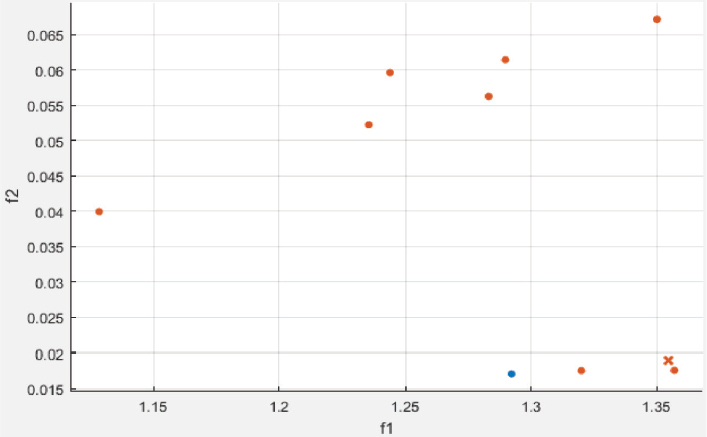
Figure 6. Scatter plot for glaucoma disease at 10 % holdout
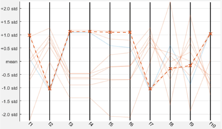
Figure 7. Parallel coordinates plot for glaucoma disease at 10 % holdout

Figure 8. Confusion matrix for glaucoma disease at 10 % holdout
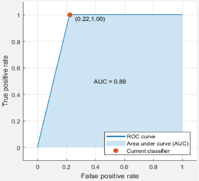
Figure 9. ROC curve for glaucoma disease at 10 % holdout
Table 2. Extracted features for 1_test.tif image
9 |
f-2 |
f-3 |
f-4 |
f-5 |
f-6 |
f-7 |
f-8 |
f-9 |
f-10 |
1.2783347 |
0.0620326 |
0.6646302 |
0.6646302 |
0.7726454 |
0.4395664 |
0.0620326 |
0.7568477 |
0.5297627 |
0.9689837 |
f-11 |
f-12 |
f-13 |
f-14 |
f-15 |
f-16 |
f-17 |
f-18 |
f-19 |
f-20 |
0.9689837 |
0.8658667 |
0.8202925 |
2.206234 |
3.2644766 |
0.486765 |
0.0620326 |
0.232524 |
-0.4037437 |
0.4848532 |
f-21 |
f-22 |
f-23 |
f-24 |
f-25 |
f-26 |
f-27 |
f-28 |
f-29 |
f-30 |
0.9793225 |
0.9875935 |
8.716128 |
9.927212 |
7.0155196 |
8.4437168 |
0.6712201 |
5.2901344 |
3.8423017 |
4.3758161 |
f-31 |
f-32 |
f-33 |
f-34 |
f-35 |
f-36 |
f-37 |
f-38 |
f-39 |
f-40 |
1.9821632 |
2.4551381 |
2.6633798 |
1.7620956 |
1.8457573 |
1.0675953 |
1.0905823 |
2.9255243 |
5.1110245 |
0.0550887 |
f-41 |
f-42 |
f-43 |
f-44 |
f-45 |
f-46 |
f-47 |
f-48 |
f-49 |
f-50 |
0.003159 |
0.0031658 |
0.008735 |
0.0102941 |
0.0081563 |
0.0090686 |
0.0081699 |
0.0064611 |
0.0079929 |
0.0102465 |
f-51 |
f-52 |
f-53 |
f-54 |
f-55 |
f-56 |
f-57 |
f-58 |
f-59 |
f-60 |
0.0098652 |
0.0117102 |
0.0085648 |
0.0104916 |
0.0070738 |
0.006216 |
0.004793 |
0.0070057 |
0.0073666 |
0.0092456 |
f-61 |
f-62 |
f-63 |
f-64 |
f-65 |
f-66 |
f-67 |
f-68 |
f-69 |
f-70 |
0.0113494 |
0.0075163 |
0.0093273 |
0.0076321 |
0.0043301 |
0.0082993 |
0.0118736 |
0.0068582 |
0.0070601 |
0.011457 |
f-71 |
f-72 |
f-73 |
f-74 |
f-75 |
f-76 |
f-77 |
f-78 |
f-79 |
f-80 |
0.0137694 |
0.0120963 |
0.0113982 |
0.0114966 |
0.0092789 |
0.0107775 |
0.0114545 |
0.0109114 |
0.011845 |
0.0100248 |
f-81 |
f-82 |
f-83 |
f-84 |
f-85 |
f-86 |
f-87 |
f-88 |
f-89 |
f-90 |
0.0101168 |
0.0107783 |
0.0095934 |
0.0084841 |
0.0097079 |
0.0088801 |
0.0096047 |
0.010433 |
0.0092358 |
0.0105486 |
f-91 |
f-92 |
f-93 |
f-94 |
f-95 |
f-96 |
f-97 |
f-98 |
f-99 |
f-100 |
0.010045 |
0.0084282 |
0.0117776 |
0.0123064 |
0.0077277 |
0.0003331 |
0.000397 |
0.0007216 |
0.0004476 |
0.0040135 |
f-101 |
f-102 |
f-103 |
f-104 |
f-105 |
f-106 |
f-107 |
f-108 |
f-109 |
f-110 |
0.0041444 |
0.0038304 |
0.0052181 |
0.0104763 |
0.00758 |
0.0094921 |
0.006728 |
0.0039446 |
0.0036584 |
0.0048196 |
f-111 |
f-112 |
f-113 |
|
|
|
|
|
|
|
0.0036479 |
0.9997612 |
0.0057761 |
|
|
GLCM |
LTE |
Tamura |
Wavelet |
LBP |
Table 3. Prediction accuracy for multi-class disease at different values of holdout
Classification method |
Recall |
Specificity |
Accuracy |
Holdout |
Linear SVM |
100 |
50 |
85.70 |
5 |
Ensemble RUSBoosted tree |
100 |
80 |
92.90 |
10 |
Fine KNN |
92.31 |
90 |
90.50 |
15 |
Cubic SVM |
88.24 |
90 |
89.70 |
20 |
Cubic SVM |
77.27 |
90 |
83.30 |
25 |
E B tree |
77.42 |
80 |
79.10 |
30 |
Table 4. Prediction accuracy for multi-class disease at different values of K-fold
Classification method |
Recall |
Specificity |
Accuracy |
K-fold cross |
Cubic SVM |
80.68 |
70 |
77.20 |
5 |
Quadratic SVM |
84.09 |
70 |
77.90 |
10 |
Quadratic SVM |
82.95 |
70 |
78.60 |
15 |
Quadratic SVM |
82.95 |
80 |
80.00 |
20 |
E B tree |
84.09 |
70 |
77.90 |
25 |
E B tree |
82.95 |
70 |
78.60 |
30 |
Table 5. Prediction accuracy for multi-class disease with enabled PCA
Classification method |
Recall |
Specificity |
Accuracy |
Holdout |
% variance |
Simple tree |
100 |
60 |
85.70 |
15 |
95 |
Logistic Regression |
84.62 |
80 |
81.00 |
15 |
90 |
Quadratic SVM |
84.62 |
90 |
85.70 |
15 |
85 |
Linear Discriminant |
83.33 |
60 |
75.90 |
20 |
95 |
Linear SVM |
94.12 |
80 |
86.20 |
20 |
90 |
KNN |
94.12 |
60 |
79.30 |
20 |
85 |
Table 6. Prediction accuracy for diabetic retinopathy at different values of holdout
Classification method |
Recall |
Specificity |
Accuracy |
Holdout |
Simple tree |
100 |
0 |
80.00 |
5 |
E B tree |
88.89 |
100 |
90.90 |
10 |
Fine KNN |
84.62 |
50 |
76.50 |
15 |
Fine Gaussian SVM |
100 |
0 |
78.30 |
20 |
Cubic SVM |
90.91 |
70 |
86.20 |
25 |
Quadratic SVM |
92.31 |
70 |
88.60 |
30 |
Table 7. Prediction accuracy for diabetic retinopathy at different values of K-fold
Classification method |
Recall |
Specificity |
Accuracy |
K-fold cross |
Cubic SVM |
89.77 |
50 |
80.00 |
5 |
Cubic SVM |
89.77 |
70 |
83.80 |
10 |
Quadratic SVM |
88.64 |
70 |
82.90 |
15 |
Quadratic SVM |
89.77 |
70 |
83.80 |
20 |
Quadratic SVM |
89.77 |
70 |
83.80 |
25 |
Quadratic SVM |
89.77 |
70 |
83.80 |
30 |
Table 8. Prediction accuracy for diabetic retinopathy with enabled PCA
Classification method |
Recall |
Specificity |
Accuracy |
Holdout |
% variance |
Medium KNN |
92.31 |
50 |
82.40 |
15 |
95 |
Medium tree |
92.31 |
50 |
82.40 |
15 |
90 |
Linear Discriminant |
100 |
0 |
76.50 |
15 |
85 |
Simple tree |
88.89 |
40 |
78.30 |
20 |
95 |
Cubic SVM |
88.89 |
40 |
78.30 |
20 |
90 |
Quadratic Discriminant |
100 |
40 |
87.00 |
20 |
85 |
Table 9. Prediction accuracy for glaucoma disease at different values of holdout
Classification method |
Recall |
Specificity |
Accuracy |
Holdout |
Linear SVM |
83.33 |
100 |
85.70 |
7 |
Simple tree |
100 |
100 |
90.00 |
10 |
Ensemble Subspace KNN |
92.31 |
100 |
93.30 |
15 |
Fine KNN |
100 |
70 |
95.00 |
20 |
Fine KNN |
90.91 |
100 |
92.00 |
25 |
Ensemble Subspace KNN |
92.31 |
100 |
93.30 |
30 |
Table 10. Prediction accuracy for glaucoma disease at different values of K-fold
Classification method |
Recall |
Specificity |
Accuracy |
K-fold |
Ensemble KNN |
89.77 |
90 |
89.30 |
5 |
Ensemble KNN |
90.91 |
90 |
90.30 |
10 |
Ensemble KNN |
93.18 |
90 |
93.20 |
15 |
Ensemble KNN |
93.18 |
90 |
93.20 |
20 |
Ensemble KNN |
90.91 |
90 |
90.30 |
25 |
Ensemble KNN |
90.91 |
90 |
90.30 |
30 |
Table 11. Prediction accuracy for glaucoma disease with enabled PCA
Classification method |
Recall |
Specificity |
Accuracy |
Holdout |
% variance |
Simple tree |
92.31 |
100 |
93.30 |
15 |
95 |
Logistic Regression |
92.31 |
50 |
86.70 |
15 |
90 |
Fine Gaussian SVM |
92.31 |
50 |
86.70 |
15 |
85 |
Simple tree |
100 |
70 |
95.00 |
20 |
95 |
Simple tree |
100 |
30 |
90.00 |
20 |
90 |
Logistic Regression |
94.12 |
30 |
85.00 |
20 |
85 |
Table 12. Prediction accuracy of glaucoma disease for RIM-ONE DL dataset
Classification method |
Recall |
Specificity |
Accuracy |
Holdout |
Ensemble RUSBoosted Tree |
100 |
70 |
87.5 |
5 |
Fine KNN |
90.91 |
100 |
94.1 |
10 |
E B tree |
88.89 |
100 |
92.3 |
15 |
Cosine KNN |
91.3 |
80 |
88.2 |
20 |
E B tree |
93.1 |
60 |
83.7 |
25 |
E B tree |
85.71 |
70 |
80.8 |
30 |
Table 13. Accuracy for different classification approaches
Authors/Year |
DR |
GC |
MCD |
85.20 |
- |
88.40 |
|
89.10 |
- |
- |
|
- |
93.5 |
- |
|
80.39 |
83.89 |
80.72 |
|
- |
89.08 |
- |
|
82.84 |
- |
- |
|
88.21 |
- |
- |
|
87.71 |
- |
- |
|
Proposed model |
90.90 |
95.00 |
92.90 |
4.4. Discussions
In the proposed model, we have used different machine learning techniques to classify retinopathy diseases. We have used holdout and k-fold cross validation methods for validation of the model. We have considered PCA enabled and disabled both perspectives. The proposed model has been experimentally verified for different values of both types of validation methods (ranging from 5 to 30 with interval 5). We have computed the recall, specificity, and accuracy for the model. We have classified glaucoma, diabetic retinopathy, and multi-class diseases. When we classify multi-class diseases then Ensemble RUSBoosted Tree reports 92.90 % accuracy at 10 % holdout. When we classify diabetic retinopathy the Ensemble Bagged Tree (E B tree) reports 90.90 % accuracy at a 10 % holdout. When we classify glaucoma then Fine KNN reports 95.00 % accuracy at 20 % holdout validation. Figure 6 shows the scatter plot where the blue dot shows glaucoma and saffron healthy features. Figure 7 shows the parallel coordinates plots where the cross dotted line shows the incorrect prediction. Here, there is only one false prediction out of ten. Figure 8 depicts the confusion matrix for the detection of glaucoma diseases at a 10 % holdout where all predictions are correct and only one prediction is a false positive prediction. Figure 9 shows the ROC curve. Here, AUC is 0.89 which is very close to 1. This validates that the accuracy of the proposed model is good. In Table 13, DR stands for diabetic retinopathy, GC for glaucoma, and MCD for multi-class diseases. In this table, we have compared various recent approaches based on machine learning and deep learning.
Machine learning methods are simple and can work better with smaller size datasets. The proposed machine learning based model has been assessed on many datasets. Therefore, the proposed approach has a lesser chance of overfitting. The segmented images are obtained after performing many operations such as preprocessing (to enhance contrast, and remove noise) and masking (to remove outliers). Preprocessing, match filtering, and masking together overcome the retinal image segmentation issues such as variability in retinal structures, low contrast, noise, and vessel characteristics. We could try to explore advanced deep learning techniques for retinal image segmentation and disease classification using both segmented and RGB images on large size different datasets.
5. Conclusion and Future Research
Critical diseases such as diabetes, glaucoma, hypertension, obesity, macular degeneration, etc. are retinopathy diseases. The proposed model is helpful for the classification of retinopathy diseases such as diabetes and glaucoma. In the proposed model, the first texture features are extracted by GLCM, LTE, Tamura, Wavelet, LBP, and HOG methods from the segmented retinal images. Thereafter, machine learning based classification is performed on the extracted features to predict glaucoma, diabetic retinopathy, and multi-class diseases. The accuracy of the proposed model for diabetic retinopathy, glaucoma, and multi-class retinal diseases is 90.90 %, 95.00 %, and 92.90 %, respectively. Experimental outcomes of the proposed model confirm that the model is proficient in identifying these retinal diseases. The proposed approach holds significant potential for practical applications in clinical settings such as early diagnosis, automated screening, improved accuracy, resource optimization, and continuous monitoring of diseases. Clinical validation and testing, integration with clinical workflows, post-deployment monitoring, etc., are the steps to move from research to implementation. In the future, we could try to explore advanced deep learning techniques for retinal image segmentation and disease classification using both segmented and RGB images on different large size datasets.
Declaration Statement
We don’t have any conflicts of interest related to this work.
References
Abitbol, E., Miere, A., Excoffier, J. B., Mehanna, C. J., Amoroso, F., Kerr, S., Ortala, M., & Souied, E. H. (2022). Deep learning based classification of retinal vascular diseases using ultra widefield color fundus photographs. BMJ Open Ophthalmology, 7(1), 1-7. https://doi.org/10.1136/bmjophth-2021-000876
Alam, M., Zhao, E. J., Lam, C. K., & Rubin, D. L. (2023). Segmentation-assisted fully convolutional neural network enhances deep learning performance to identify proliferative diabetic retinopathy. Journal of Clinical Medicine, 12(1). https://doi.org/10.3390/jcm12010001
Attia, A., Akhtar, Z., Akhrouf, S., & Maza, S. (2020). A survey on machine and deep learning for detection of diabetic retinopathy. Image and Video Processing, 11(2), 2337-2344. https://doi.org/10.1007/s11042-020-08625-1
Batista, F., & José, F. (2020). A unified retinal image database for assessing glaucoma using deep learning. Image Analysis & Stereology, 39(3), 161-167. https://doi.org/10.5566/ias.2210
Boser, E. B., Guyon, M. I., & Vapnik, N. V. (1992). A training algorithm for optimal margin classifiers. In Proceedings of the fifth annual workshop on Computational Learning Theory-COLT (pp. 144-152). https://doi.org/10.1145/130385.130401
Cao, J., Chen, J., Zhang, X., Yan, Q., & Zhao, Y. (2022). Attentional mechanisms and improved residual networks for diabetic retinopathy severity classification. Journal of Healthcare Engineering, 1-10. https://doi.org/10.1155/2022/1234567
Cortes, C., & Vapnik, V. (1995). Support-vector networks. Machine Learning, 20(3), 273-297. https://doi.org/10.1007/BF00994018
Cover, T. M., & Hart, E. P. (1967). Nearest neighbor pattern classification. IEEE Transactions on Information Theory, 13(1), 21-27. https://doi.org/10.1109/TIT.1967.1053964
Das, A., Giri, R., Chourasia, G., & Bala, A. A. (2019). Classification of retinal diseases using transfer learning approach. In Proceedings of the Fourth International Conference on Communication and Electronics Systems (pp. 2075-2079). Coimbatore, India. https://doi.org/10.1109/ICCES.2019.8924101
Fisher, R. A. (1936). The use of multiple measurements in taxonomic problems. Annals of Eugenics, 7(2), 179-188. https://doi.org/10.1111/j.1469-1809.1936.tb02137.x
Fix, E., & Hodges, J. (1951). Discriminatory analysis. Non-parametric discrimination: Consistency properties. USAF School of Aviation Medicine, Randolph Field, Texas. https://doi.org/10.21236/AD0246377
Gour, N., & Khanna, P. (2021). Multi-class multi-label ophthalmological disease detection using transfer learning based convolutional neural network. Biomedical Signal Processing and Control, 66, 1-8. https://doi.org/10.1016/j.bspc.2021.102492
Han, Y., Li, W., Liu, M., Wu, Z., Zhang, F., Liu, X., Tao, L., Li, X., & Guo, X. (2021). Application of an anomaly detection model to screen for ocular diseases using color retinal fundus images: Design and evaluation study. Journal of Medical Internet Research, 23(7), 1-12. https://doi.org/10.2196/23456
Haralick, R. M., Shanmugam, K., & Dinstein, I. (1973). Textural features for image classification. IEEE Transactions on Systems, Man, and Cybernetics, 3(6), 610-621. https://doi.org/10.1109/TSMC.1973.4309314
Hoover, A., Kouznetsova, V., & Goldbaum, M. (2000). Locating blood vessels in retinal images by piecewise threshold probing of a matched filter response. IEEE Transactions on Medical Imaging, 19(3), 203-210. https://doi.org/10.1109/42.845178
Jiang, H., Yang, K., Gao, M., Zhang, D., Ma, H., & Qian, W. (2019). An interpretable ensemble deep learning model for diabetic retinopathy disease classification. In 41st Annual International Conference of the IEEE Engineering in Medicine and Biology Society (EMBC) (pp. 2045-2048). https://doi.org/10.1109/EMBC.2019.8857745
Juneja, M., Thakur, S., Uniyal, A., Wani, A., Thakur, N., & Jindal, P. (2022). Deep learning-based classification network for glaucoma in retinal images. Computers and Electrical Engineering, 101. https://doi.org/10.1016/j.compeleceng.2022.107995
Korkmaz, S. A., Akçiçek, A., Bínol, H., & Korkmaz, M. F. (2017). Recognition of the stomach cancer images with probabilistic HOG feature vector histograms by using HOG features. In 15th International Symposium on Intelligent Systems and Informatics (SISY) (pp. 000339-000342). https://doi.org/10.1109/SISY.2017.8080563
Laws, K. (1980). Rapid texture identification. Image Processing for Missile Guidance, 238, 376-380. https://doi.org/10.1117/12.959774
Li, T., Gao, Y., Wang, K., Guo, S., Liu, H., & Kang, H. (2019). Diagnostic assessment of deep learning algorithms for diabetic retinopathy screening. Information Sciences, 501, 511-522. https://doi.org/10.1016/j.ins.2019.06.011
Londhe, M. (2021). Classification of eye diseases using hybrid CNN-RNN models. MSc Project, National College of Ireland, 1-20. https://doi.org/10.1109/ICCMC.2021.9763803
Mallat, S. (1989). Multifrequency channel decomposition of images and wavelet models. IEEE Transaction on ASSP, 37(12), 2091-2110. https://doi.org/10.1109/29.45599
McLachlan, G. J. (2004). Discriminant analysis and statistical pattern recognition. Wiley Interscience. ISBN 978-0-471-69115-0. https://doi.org/10.1002/0471725293
Muchuchuti, S., & Viriri, S. (2023). Retinal disease detection using deep learning techniques: A comprehensive review. Journal of Imaging, 9(84), 1-38. https://doi.org/10.3390/jimaging9080084
Nazir, T., Nawaz, M., Rashid, J., Mahum, R., Masood, M., Mehmood, A., Ali, F., Kim, J., Kwon, H.-Y., & Hussain, A. (2021). Detection of diabetic eye disease from retinal images using a deep learning based CenterNet model. Sensors, 21(16), 1-18. https://doi.org/10.3390/s21165528
Odstrcilik, J., Kolar, R., Budai, A., Hornegger, J., Jan, J., Gazarek, J., Kubena, T., Cernosek, P., Svoboda, O., & Angelopoulou, E. (2013). Retinal vessel segmentation by improved match filtering: Evaluation on a new high resolution fundus image database. IET Image Processing, 7(4), 373-383. https://doi.org/10.1049/iet-ipr.2012.0455
Ojala, T., Pietikainen, M., & Maenpaa, T. (2002). Multi-resolution grayscale and rotation invariant texture classification with local binary patterns. IEEE Transactions on Pattern Analysis and Machine Intelligence, 24(7), 971-987. https://doi.org/10.1109/TPAMI.2002.1017623
Opitz, D., & Maclin, R. (1999). Popular ensemble methods: An empirical study. Journal of Artificial Intelligence Research, 11, 169-198. https://doi.org/10.1613/jair.614
Pin, K., Chang, J. H., & Nam, Y. (2022). Comparative study of transfer learning models for retinal disease diagnosis from fundus images. Computers, Materials & Continua, 70(3), 5821-5834. https://doi.org/10.32604/cmc.2022.021583
Pinto, A.-D., Morales, S., Naranjo, V., Köhler, T., Mossi, J. M., & Navea, A. (2019). CNNs for automatic glaucoma assessment using fundus images: An extensive validation. BioMedical Engineering OnLine, 18, 29, 1-19. https://doi.org/10.1186/s12938-019-0652-5
Qin, C., & Siang, S. (2016). An efficient method of HOG feature extraction using selective histogram bin and PCA feature reduction. Advances in Electrical and Computer Engineering, 16(4), 101-108. https://doi.org/10.4316/AECE.2016.04013
Quinlan, J. R. (1986). Induction of decision trees. Machine Learning, 1, 81-106. https://doi.org/10.1007/BF00116251
Rokach, L. (2010). Ensemble-based classifiers. Artificial Intelligence Review, 33(1-2), 1-39. https://doi.org/10.1007/s10462-009-9124-7
Rokach, L., & Maimon, O. (2014). Data mining with decision trees: Theory and applications. 2nd Edition, World Scientific Publishing Co Inc, 69, 1-244. https://doi.org/10.1142/9789814590090
Sarki, R., Ahmed, K., Wang, H., & Zhang, Y. (2020). Automated detection of mild and multi-class diabetic eye diseases using deep learning. Health Information Science and Systems, 8(1), 1-9. https://doi.org/10.1007/s13755-020-00111-8
Saroj, S. K., Kumar, R., & Singh, N. P. (2020). Fréchet PDF based matched filter approach for retinal blood vessels segmentation. Computer Methods and Programs in Biomedicine, 194, 1-17. https://doi.org/10.1016/j.cmpb.2020.105515
Saroj, S. K., Kumar, R., & Singh, N. P. (2022). Retinal blood vessels segmentation using Wald PDF and MSMO operator. Computer Methods in Biomechanics and Biomedical Engineering: Imaging & Visualization, 10(2), 1-18. https://doi.org/10.1080/21681163.2021.1989467
Saroj, S. K., Ratna, V., Kumar, R., & Singh, N. P. (2020). Efficient kernel based matched filter approach for segmentation of retinal blood vessels. Solid State Technology, 63(5), 7318-7334. https://doi.org/10.1016/j.sst.2020.05.001
Sengar, N., Joshi, R. C., Dutta, M. K., & Burget, R. (2023). EyeDeep-Net: A multi-class diagnosis of retinal diseases using deep neural network. Neural Computing and Applications, 35, 1-21. https://doi.org/10.1007/s00521-022-07345-1
Shrivastava, A., Kamble, R., Kulkarni, S., Singh, S., Hegde, A., Kashikar, R., & Das, T. (2021). Deep learning based ocular disease classification using retinal fundus images. Investigative Ophthalmology & Visual Science, 63(11). https://doi.org/10.1167/iovs.63.11.1
Staal, J., Abramoff, M. D., Niemeijer, M., Viergever, M. A., & Ginneken, B. V. (2004). Ridge based vessel segmentation in color images of the retina. IEEE Transaction on Medical Imaging, 23(4), 501-509. https://doi.org/10.1109/TMI.2004.825627
Tamura, H., Mori, S., & Yamawaki, T. (1978). Textural features corresponding to visual perception. IEEE Transactions on Systems, Man, and Cybernetics, 8(6), 460-473. https://doi.org/10.1109/TSMC.1978.4309999
Tolles, J., & Meurer, J. W. (2016). Logistic regression relating patient characteristics to outcomes. JAMA, 316(5), 533-534. https://doi.org/10.1001/jama.2016.7653
Virmani, J., Singh, G. P., Singh, Y., & Kriti. (2019). PNN-based classification of retinal diseases using fundus images. Sensors for Health Monitoring, 5, 215-242. https://doi.org/10.3390/s1909215
Zhu, S., Lu, B., Wang, C., Wu, M., Zheng, B., Jiang, Q., Wei, R., Cao, Q., & Yang, W. (2022). Screening of common retinal diseases using six-category models based on EfficientNet. Frontiers in Medicine, 9, 1-9. https://doi.org/10.3389/fmed.2022.1234567