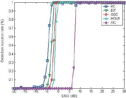
Figure 1: Statistical performance with two targets.
ADCAIJ: Advances in Distributed Computing and Artificial Intelligence Journal
Regular Issue, Vol. 13 (2024), e31710
eISSN: 2255-2863
DOI: https://doi.org/10.14201/adcaij.31710
Yuhong Yina, Qian Jiab, Huiqi Xuc and Guanglei Fudd
a School of Electronic Engineering, Xi’an Aeronautical Institute, Xi’an, China
b School of Economics, Xi’an University of Finance and Economics, Xi’an, China
c School of Automation, Northwestern Polytechnical University, Xi’an, China
d Engineering Practice Training Center, Northwestern Polytechnical University, Xi’an, China
59763537@qq.com, jiaqianxd@163.com, h.q.xu@mail.nwpu.edu.cn, fugl@nwpu.edu.cn
ABSTRACT
This paper studies five classic multi-target detection methods in different noisy environments, including Akaike information criterion, ration criterion, Rissanen’s minimum description length, Gerschgorin disk estimator and Eigen-increment threshold methods. Theoretical and statistical analyses of these methods have been done through simulations and a real-world water tank experiment. It is known that these detection approaches suffer from array errors and environmental noises. A new diagonal correction algorithm has been proposed to address the issue of degraded detection performance in practical systems due to array errors and environmental noises. This algorithm not only improves the detection performance of these multi-target detection methods in low signal-to-noise ratios (SNR), but also enhances the robust property in high SNR scenarios.
KEYWORDS
multi-target detection; diagonal amendatory; noise estimator; information theoretic criteria
A sensor network is a set of geographically dispersed, interconnected sensors and can cooperatively handle highly complex tasks such as tracking a time varying number of targets (Casado-Vara et al., 2019; Li et al., 2019a; Li et al., 2019b). With the development of sensor networks, object detection technology can obtain more accurate data information, and obtains the target details through data analysis, processing or artificial intelligence (Hussain et al., 2022a) and other methods (Muhamada and Mohammed, 2022). Object detection technology has been widely used in military and civilian fields, such as multi-target tracking and automatic driving (Qader Kheder and Aree Ali, 2023; Hussain et al., 2022b).
Decentralized signal and information processing over sensor network has played an important role in both academic study and many engineering problems, such as the multi-sensor target detection and tracking in clutter and noisy environments (Sayed, 2014; Meyer et al., 2018; Li et al., 2023b). Lying in the center of this research topic, the array signal processing has been rapidly developed in recent decades, which aims at obtaining some characteristics of the signal, such as direction of arrival (DOA), frequency, etc (Jiang and Zhou, 2023). DOA is closely related to the azimuth, angel and bearing measurements. The super-resolution DOA estimation is an important research topic, involving communication, radar, sonar, seismic exploration and other fields (Yang and Han, 2013; Van Trees, 2002; Li et al., 2023c). Among many signal processing applications, the problem of signal source number estimation (SSNE) plays a key role, since it is the prerequisite for the super-resolution DOA estimation. If the SSNE can not be accurately solved, the performance of the DOA estimation algorithm drops sharply, or even fails completely.
The study of SSNE in array signal processing can be dated back to 1950s and 1960s (Liu and Liao, 2004), when it was originally addressed via hypothesis testing. Since the hypothesis testing method needs to manually determine a detection threshold for comparison with the likelihood ratio test statistic, it is easily affected by human subjective factors, which can cause significant estimation errors. In the past several decades, many approaches have been proposed based on statistical information, Bayesian criterion, or approximate maximum likelihood ratio, etc. Wax and Kailath (1985) first introduced information theory criteria into array signal processing to solve the problem of SSNE. They gave the Akaike information criterion (AIC) (Akaike, 1974) and minimum description length (MDL) criterion (Wax and Ziskind, 1989; Karhunen et al., 1997) in the form of the eigenvalues of the array covariance matrix, which is user-friendly and overcomes the shortcomings of the hypothesis testing. However, the AIC does not have the feature of consistent estimation. Even in the case of high signal-to-noise ratios (SNR) and large snapshots, it still has a large error probability. Although MDL belongs to consistent estimation, the performance loss is severe in a low SNR environment, and the problem of underestimation of the number of signals may occur (Wan et al., 2020). Following this thinking, many scholars proposed a variety of improved SSNE methods based on information theory criteria (Wei et al., 2015; De Ridder et al., 2005). Zhao et al. (1986; 1987) gave a method called the effective detection criterion (EDC), proved the strong consistency of the criterion, and pointed out that the MDL standard is a special case of the EDC rule. Wong and Reilly (1990) applied a new logarithmic likelihood function to the AIC criterion and the MDL criterion, leading to the revised AIC criterion and the MDL criterion, respectively. Fisher and Messer (1999; 2000) gave an MDL criterion based on order statistics (OSMDL), which has a better performance than the MDL criterion, but at the cost of a higher computational complexity. The well-known eigenvalue method proposed by Chen and Reilly can be viewed as a specific variant of the technique that uses the one-step prediction of the eigenvalues to get the SSNE (Chen et al., 1991), which predicts the upper limit of the noise characteristic value, and obtains the SSNE according to the comparison result of the estimated characteristic value and the predicted value. The ration criterion (RC) was proposed by Wang and Huang (1996), which avoids the drawback of high estimation of signal numbers in the traditional information criteria methods. Wax and Ziskind further proposed a detection algorithm based on the signal subspace and the noise subspace, called based on Rissanen’s Minimum description length (MDLB) (Wax and Ziskind, 1989), which can solve the detection problem of related signals. Olivia, Hu et al. proposed an Eigen-increment threshold (EIT) algorithm with promising applications by studying the potential characteristics of the array covariance matrix noise eigenvalue (Hu et al., 1999).
The above estimation methods are only applicable to the white noise environment. However, in actual engineering projects or various complex interference electromagnetic environments, it is difficult for the white noise model to meet various requirements. Often mixture models or heavy-tailed models are used for modeling complicated noises (Li et al., 2019c; Li et al., 2023a), which often poses a higher computation requirement. In order to solve this problem, the Gerschgorin disk theorem (GDE) was proposed by Wu et al. (1995), which does not need to accurately calculate the eigenvalues of the received data matrix. It is only necessary to use the GDE to estimate the position of each eigenvalue and finally obtain the number of signal sources. Although the GDE method can work well in the colored noise environment and can more accurately detect source numbers, the threshold of the method requires a subjective adjustment factor. The inappropriate selection of the adjustment factor leads to large estimation errors.
In the real-world system, due to the influence of the array error and environmental non-white noise, the detection performance of the above mentioned algorithms is significantly reduced. To solve this problem, this paper proposes a diagonal correction algorithm to improve the detection performance and robustness of the multi-target detection algorithm.
The structure of this paper is organized as follows. Section 2 introduces the basic theory of array signal processing, that is, the mathematical model of the DOA estimation. Section 3 introduces the traditional signal source number estimation algorithms. Section 4 proposes our diagonal correction method. The experimental results are presented in Section 5. Concluding observations are given in Section 6.
Denoting the number of array elements by M and the number of signal sources by q, the array receiving vector can be expressed as:
where A = [a(θ1), … , a(θq)] is the M × q-dimensional orientation matrix, a(θi) is an M × 1-dimensional steering vector determined by the array structure and the unknown parameters of the i-th signal, sT(t) = [s1(t), … , sq(t)] is a q × 1-dimensional signal vector, and n(·) is an M × 1-dimensional noise complex vector.
In this paper, we assume q < M, and s1(·), … , sq(·) is a complex Gaussian random process with zero mean and positive definite covariance matrix.
The Gaussian white noise and colored noise models are used (Akaike, 1974). The noise vector n(·) is a complex Gaussian random vector with zero mean and a covariance matrix of σ2I, where σ2 is an unknown scalar, I is an identity matrix, and the noise is independent of the signal.
In general, colored noise is obtained by the Gaussian white noise filtering, whose vector is as follows:
where ξ(t) is white Gaussian noise, and λ is the correlation time. The spatial color noise intensity is 2D, and the color noise autocorrelation function is:
The expression of the elements of the noise covariance matrix in the colored noise model (Stoica and Cedervall, 1997) is given by as follows:
where σ2n is the power of colored noise, ρ is the correlation coefficient of adjacent array elements receiving noise, ρ=0 means that the received noise is Gaussian white noise.
According to the white noise background, the covariance matrix of the array received signal can be obtained from Eq. 1.
where S = E[s(·)s(·)H] is the source covariance matrix, and E represents the mathematical expectation.
Assume that the array direction matrix A has full column rank, that is, the column vector of A(θi)(i = 1, … , q) is linearly independent. The source covariance matrix S is non-singular, then the rank of the matrix A(θ)SA(θ)* is q, and the M − q small eigenvalues of A(θ)SA(θ)* are zero. Without loss of generality, we assume λ1 ≥ λ2 ≥ … λM which are the eigenvalues of the array covariance matrix R, and the M − q smallest eigenvalues of R are equal to σ2, namely:
Therefore, the number q of signal sources can be determined by the number of small eigenvalues of the array covariance matrix R. But in practice, the array covariance matrix R cannot be obtained accurately, and can only be estimated by using a limited number of the array snapshot data. The eigenvalues of the array covariance matrix estimated from finite snapshot data no longer have the property described by Eq. 6, that is, the small eigenvalues (noise eigenvalues) are no longer equal, but have a relationship with probability 1.
Therefore, under the condition that only limited snapshot data is available, the number of signal sources cannot be determined according to the number of small eigenvalues of the array covariance matrix.
Both the AIC (Akaike, 1974) and the MDL criterion (Wax and Ziskind, 1989) are the method for solving the model selection problem. The problem solved by the criterion of information theory is given by a set of observed data X = [x(1), … , x(N)] and a series of parameterized probability models f(x∣Θ), where Θ represents the parameter vector of the probability model, through selecting the model that best fits the observed data.
The model proposed by Akaike aims to minimize the AIC. The definition of this information-theoretic criterion is expressed by the following equation:
where -logf(∣Θ^) represents the maximum log-likelihood function term, and 2k represents the penalty function term.
The estimation of the number of signal sources can be achieved using information theory criteria, and the AIC criterion for the estimated number of signal sources can be obtained through calculation as follows:
The first term in the above formula is the log-likelihood function term of the maximum likelihood estimation of the model parameters, and the second term is the penalty function term. The k that minimizes Eq. (9) is the number of signals that have been detected by the AIC criterion.
The introduction of information criteria is aimed for solving the problem of order determination in the autoregressive model (AR). Due to the existence of noises, theoretically, the higher the order of the AR model, the higher the approximation accuracy of the actual signal. Therefore, the order of the model is easily overestimated by the information criterion. The same issue of overestimation can arise when using information criteria to determine the number of signals, which can result in estimation bias.
Based on the information criterion such as the AIC and the MDL, the RC can efficiently suppress over-estimation. An AIC-based ration criterion is proposed as follows:
The k that minimizes Eq. (10) is the number of signals that have been detected by the AIC. The RC criterion can suppress the over-estimation of the information criterion for the number of signals and obtain a better estimation effect.
The vector received by the array x(t) can be decomposed into the signal subspace and the noise subspace, which is expressed as follows:
where xS(t) denotes the k ×1 component in the signal subspace, xN(t) denotes the (q −k) ×1 component in the noise subspace, and G(θ(k))) denotes a unitary coordinate transformation matrix, determined so as to satisfy the relations:
and
Here and denote the projection matrices on the signal and noise subspaces, respectively,
By using the MDL criterion and the encoding of the data sequence by the signal subspace model, we can get the code size of the noise subspace and the signal subspace. By combining the invariance and certainty criteria of matrix trace, the expression of signal azimuth estimation can be obtained as follows:
where li(θ(k) ≥ … ≥ l(p−k) (θ(k)) denote the nonzero eigenvalue of the p × p matrix . More details of reasoning can be found in reference (Wax and Ziskind, 1989).
Eq.(16) involves a multi-dimensional search over the azimuth angles of the signal sources, and at each iteration of the search, the matrix eigen decomposition needs to be carried out to estimate the signal subspace. This can be computationally intensive, especially when the number of signal sources or the dimensionality of the search space is high. This paper employs a relatively simple and effective alternating projection algorithm which can save computation (Strang, 2006). Substituting the estimated azimuth angle into Eq. (16), according to the MDLB criterion, we have
The k that minimizes Eq. (17) is the number of signals that have been detected by the proposed MDLB. This method can estimate the azimuth angle of the signal while detecting the number of targets.
The eigenvalues of the array covariance matrix R are described in the Eq. (7) and define λi − λi+1(i =1, 2, ...M) as the eigenvalue increments. The q signal eigenvalues are randomly added to the noise eigenvalues, thus destroying the linear relationship of the noise eigenvalues. This leads to an increase in the feature increment at the boundary of the two subspaces (signal and noise subspaces), and a threshold can be set to detect this increase. A single eigenvalue increment detection algorithm is proposed as follows:
where is the signal power, η(M,N) is a coefficient function and the following conditions are satisfied:
• When N → ∞, η(M,N) = 1.
• When N decreases, η(M,N) increases.
• When M increases, η(M,N) decreases.
Where i is the number of detected signals when Eq. (18) is not satisfied.
Since the information of the noise eigenvalues is directly introduced into this theory, this criterion greatly reduces the influence of errors and has a small bias performance. When this estimation is used in subspace-based signal processing, the computational complexity can be ignored, which makes it earn good engineering application prospects.
The GDE criterion first transforms the covariance matrix into a partitioned matrix (Li et al., 2021), as follows:
where R' is the sub-matrix of R after removing the last row and the last column, using its eigenspace (eigenmatrix U, satisfying UUH = 1 and R′ = UΣU) to construct a unitary matrix T:
Performing a unitary transformation of the covariance matrix:
where λi is the center of Gerschgorin disk, and the first M −1 erschgorin radius of the matrix RT is:
where, AM−1 is the array manifold, RS is the source matrix, and bM is the steering vector. Obviously, has no relation with i, so the Gerschgorin radius is only affected by . Due to the orthogonality between the noise vector and the steering vector, when ei corresponds to the noise vector, the Gerschgorin radius is small, in other cases, the radius is larger.
Through the above transformation, the Gerschgorin circles of the array covariance matrix can be divided into two distinct groups. The criterion for estimating the number of signals using the radius of the Gerschgorin circle is:
where N is the number of snapshots, and D(N) is the decreasing function between 0 and 1 with respect to N, assuming the first negative value of GDE(k) is GDE(ˆk), then the SSNE is ˆq = ˆk −1.
It can be seen from the expression of the Gerschgorin disk criterion that the criterion value GDE(k) is the difference between the radius k of the k-th Gerschgorin disk and a certain threshold value. The threshold value is the average of all M − 1 Gerschgorin disk radii multiplied by an adjustment factor D(N). Specifically, it involves comparing the radius of the Gerschgorin disks associated with the transformed covariance matrix to a predefined threshold value. Based on the outcome of this comparison, the criterion enables the determination of the number of signal sources present in the system.
Due to the influence of array errors and non-white noise in the environment, the detection performance of the aforementioned array signal processing algorithms may significantly degrade. To improve the performance of the algorithm in this situation, we propose a computationally efficient solution, referred to as the diagonal correction.
At the core of our approach, the diagonal correction algorithm aims to compensate for errors that may arise in the array autocorrelation matrix, which can adversely affect signal detection. By adding a correction term to the diagonal elements of the matrix, the algorithm seeks to improve the accuracy and robustness of signal detection in the presence of such errors. This correction term is equivalent to adding strict spatial white noise to the array input signal, which can reduce the influence of array errors on the signal detection performance. The selection of the correction term needs to balance the detection performance under the low and high SNR, and should not be too large to avoid affecting the performance under low SNR, or too small to fail to achieve the effect of shielding array errors. The diagonal correction is defined as follows:
where R′ represents the matrix resulting from the addition of a correction term to the diagonal of R, while β denotes the correction applied by the algorithm. Importantly, it is worth noting that the adjustment of β does not alter the eigenvectors of the matrix, but rather influences its eigenvalues. Specifically, μi and λi represent the eigenvalues of R′ and R, respectively, and the appropriate selection of β can greatly impact the relative magnitudes of these eigenvalues, thereby affecting the performance of the algorithm in detecting signals amidst background noise.
In practice, the correction factor β is typically used to adjust the magnitude of the correction term, thereby achieving a balance between detection performance under low and high SNR conditions. However, it is important to note that the optimal size of the correction term may vary depending on the specific application and the characteristics of the input data. Therefore, it is necessary to carefully calibrate and optimize the correction term to achieve the best possible detection performance in a given scenario.
The advantages of the diagonal correction algorithm are its simplicity, ease of implementation, and effectiveness in mitigating the impact of array errors on the signal detection performance. Moreover, this algorithm does not require any assumption on the distribution of signal and noise, and can be applied to any signal and noise distribution.
The primary concept behind applying the diagonal loading technique to the array covariance matrix is to introduce a fixed correction term to the diagonal elements of the matrix. This correction term reduces the impact of colored noise on the eigenvalues, much like white noise at a fixed power level. Divergence problems can be reduced and algorithm performance improved by changing the diagonal loading’s magnitude. There are a few important factors to consider while figuring out the ideal loading factor. The algorithm’s performance in low SNR circumstances may suffer if the loading factor is set very high. On the other hand, if the loading factor is set too low, the eigenvalues may not be smoothed down as planned.
Therefore, choosing the right loading factor can be difficult. It is a challenging task to determine the loading factor’s mathematically ideal value. As a result, this part uses the analysis that follows to suggest an acceptable loading factor value.
If there is only one signal source in the space and the spatial noise is Gaussian colored noise, the M eigenvalues of the covariance matrix R of the observed data sample will ideally satisfy the following relationship, λ1 > λ2 > … λM, where λi represents the eigenvalue. In this scenario, a power parameter β is introduced to the sensor array, representing the white noise component. It is important to note that β ≪ λ1. On the other hand, to effectively mitigate the divergence of eigenvalues induced by colored noise, it is necessary to ensure that β > λM. When the signal-to-noise ratio SNR is very large, the empirical formula is as follows:
The condition is satisfied when λM ≪ β ≪ λi. The enhanced algorithm provides consistent estimations and exhibits superior performance in both low and high SNR scenarios.
In this section, simulation is used to verify the effectiveness of the proposed method and compare its performance with that of existing algorithms. In our simulations, assume that the uniform line antenna array contains 14 elements with an array spacing of half a wavelength and the noise is Gaussian white noise. There are two and three independent signals with equal power in space, and the initial phase is zero. A beam width (BW) is approximately 7.2°, the signal azimuth interval is 1/2BW, the number of snapshots is N= 500, and the change of SNR ranges from -20dB to 30dB. 100 Monte Carlo experiments are performed at each SNR to calculate the detection performance.
We discuss the impact of different SNR on the estimation performance of each algorithm. The simulation curves in white noise background are shown in Figure 1 and Figure 2 for the scenarios of two and three targets, respectively. Upon analyzing Figures 1-2, it becomes apparent that when dealing with a white noise model and a limited sample size, all five methods demonstrate effective estimation of the number of sources. Among these methods, the RC algorithm exhibits superior performance, followed by EIT (ƞ=2.5) and GDE (D(N)=1). In contrast, AIC scores the worst when measured against EIT and MDLB. All five techniques exhibit improved estimating performance as the SNR of the Gaussian white noise increases. Nevertheless, these approaches' estimating performance tends to deteriorate with increasing source count.
Figure 1: Statistical performance with two targets.
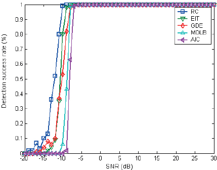
Figure 2: Statistical performance with three targets.
As shown in Figures 3-4, the detection probability of different approaches varies with the SNR when Gaussian colored noise is present in the channel. Here, the noise correlation coefficient, denoted as ρ, takes values of 0.3 and 0.7, respectively. It can be observed that the detection performance of the aforementioned algorithms diminishes in the presence of colored noise. Specifically, the detection performance of the algorithms degrades under low SNR situations as the noise correlation coefficient ρ grows. However, across a range of correlation values, the RC and EIT algorithms provide comparatively strong detection performance. In Figure 3, when the SNR is greater than -2dB, the RC and EIT algorithms achieve estimation accuracies of 1. On the other hand, the AIC algorithm demonstrates poor detection capability, requiring an SNR greater than 27dB to achieve a detection probability of 1.
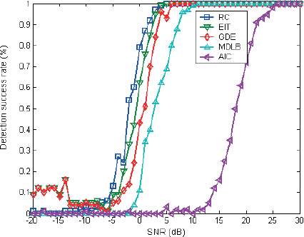
Figure 3: Statistical performance at ρ=0.3.
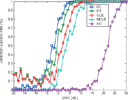
Figure 4: Statistical performance at ρ=0.7.
To investigate the performance of the above algorithms in the real-world system, we have carried out the corresponding multi-target detection underwater experiment. The receiving array consists of a 14-element uniform linear array, and the transmitted signal is a continuous sinusoidal wave. Due to the limitations of the experimental condition, the noise received in the experiment is isotropic white Gaussian noise and colored noise generated by computer simulation.
(1) Analysis of spatial white Gaussian noise
To perform a statistical study on the technique outlined above, we used anechoic pool test data from two targets with actual azimuth angles of [-6.36°, -2.84°] (azimuth interval of 0.48BW). The findings, which are shown in Figure 5, show that under high SNR circumstances, detection performance decreases for both the AIC and the MDLB criteria. After careful investigation, we have concluded that this phenomenon is not caused by array element correlation. Additional examination has demonstrated that array mistakes are to blame for the performance decline. In particular, the noise subspace’s eigenvalues show notable divergence at high SNR levels. Consequently, the ratio of eigenvalues between the signal subspace and the larger eigenvalues of the noise subspace is relatively small compared to the ratio between the larger and smaller eigenvalues of the noise subspace. This discrepancy leads to overestimation in certain algorithms, resulting in a decline in detection performance.
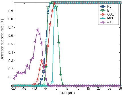
Figure 5: Statistical performance before correction.
We include the diagonal loading adjustment as suggested in Section 4 to improve the accuracy of the previously mentioned algorithm in determining the number of signal sources. This correction enables us to account for the algorithm’s detection performance under varying SNR. The amount of correction can be efficiently adjusted to accommodate both high and low SNR by varying the parameter β.
From Figure 6 to Figure 10, it is apparent that the correction factor β has a significant impact on the performance of the diagonal loading correction algorithm. When β is excessively large, as depicted in Figure 6, the algorithm’s detection performance deteriorates under low SNR conditions. Conversely, if β is too small, as illustrated in Figure 10, the diagonal loading correction algorithm fails to mitigate array errors effectively. By analyzing the statistical results, it can be concluded that β=0.02 yields relatively better detection performance under low SNR conditions while significantly improving robustness under high SNR situations. Thus, it is recommended to set the correction factor β within the range of 0.005 to 0.02 based on the analysis of different correction quantities.
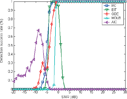
Figure 6: Statistical performance of β=0.1.
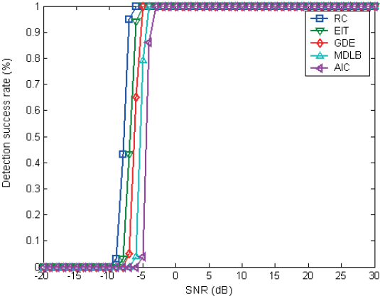
Figure 7: Statistical performance of β=0.05.
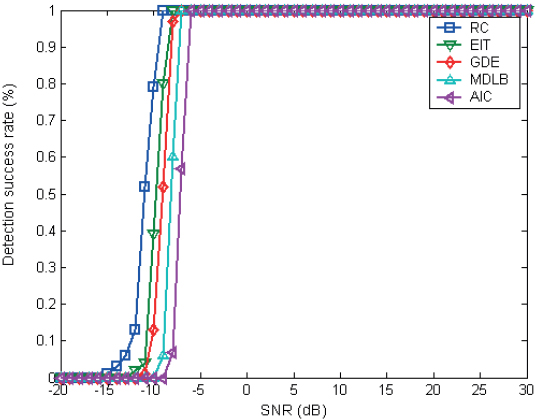
Figure 8: Statistical performance of β=0.02.
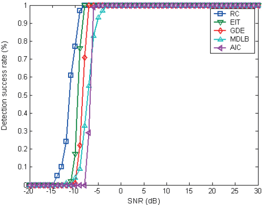
Figure 9: Statistical performance of β=0.005.
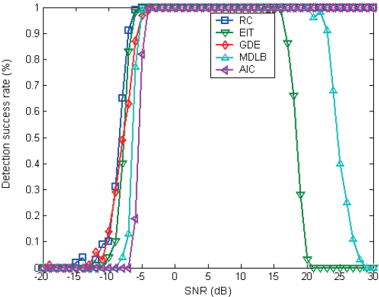
Figure 10: Statistical performance of β=0.003.
(2) Analysis of spatial non-white noise
By selecting a suitable correction factor, the diagonal loading correction algorithm exhibits good performance in white noise background. A large number of statistical simulation results have shown that this correction algorithm also performs well in correcting colored white noise background.
Under the background of colored white noise, the above algorithm was corrected with diagonal loading using the experimental data. The statistical performance of the algorithm was analyzed with noise correlation coefficients of ρ=0.3 and 0.7, as shown in Figure 11 and Figure 12, respectively, with the correction factor β set to 0.02.
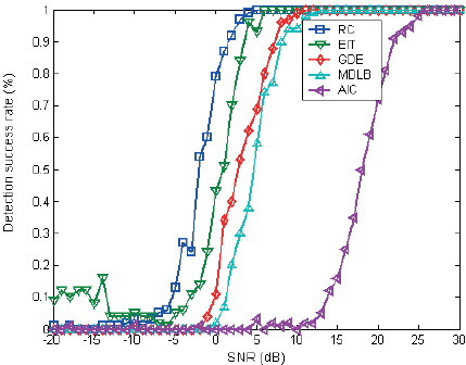
Figure 11: The performance of ρ=0.3 after revision.

Figure 12: The performance of ρ=0.7 after revision.
Compared with the simulation results in Figure 3 and Figure 4, the modified results in Figure 11 and Figure 12 show that the performance of the above algorithm has been improved after diagonal loading correction, and its detection performance is basically close to the result of the computer simulation. Thus, the effectiveness of the diagonal loading correction algorithm can be verified.
The diagonal correction algorithm is proposed to address the problem of the performance degradation in multi-target detection algorithms caused by the array error and environmental noise. Through the statistical performance analysis and the water tank test data validation under different corrections and different noisy environments, the results show that the diagonal correction algorithm improves the detection performance under the low SNR, improves the robustness under the high SNR, and provides an effective means of applying multi-target detection in engineering.
Future research can further explore and optimize the diagonal correction algorithm to meet the multi-target detection requirements in different scenarios. Additionally, a better understanding and processing of the array error and environmental noise can further enhance the performance and practicality of multi-target detection algorithms.
Akaike, H., 1974. A new look at the statistical model identification. IEEE transactions on automatic control, 19(6):716-723.
Casado-Vara, R., Novais, P., Gil, A. B., Prieto, J., and Corchado, J. M., 2019. Distributed Continuous-Time Fault Estimation Control for Multiple Devices in IoT Networks. IEEE Access, 7:11972-11984. doi: 10.1109/ACCESS.2019.2892905.
Chen, W., Wong, K. M., and Reilly, J. P., 1991. Detection of the number of signals: A predicted eigen-threshold approach. IEEE Transactions on Signal Processing, 39(5):1088-1098.
De Ridder, F., Pintelon, R., Schoukens, J., and Gillikin, D. P., 2005. Modified AIC and MDL model selection criteria for short data records. IEEE Transactions on Instrumentation and Measurement, 54(1):144-150.
Fishler, E. and Messer, H., 1999. Order statistics approach for determining the number of sources using an array of sensors. IEEE Signal Processing Letters, 6(7):179-182.
Fishler, E. and Messer, H., 2000. On the use of order statistics for improved detection of signals by the MDL criterion. IEEE Transactions on Signal Processing, 48(8):2242-2247.
Hu, O., Zheng, F., and Faulkner, M., 1999. Detecting the number of signals using antenna array: a single threshold solution. In ISSPA'99. Proceedings of the Fifth International Symposium on Signal Processing and its Applications (IEEE Cat. No. 99EX359), volume 2, pages 905-908. IEEE.
Hussain, A., Ahmad, M., Hussain, T., and Ullah, I., 2022a. Efficient Content Based Video Retrieval System by Applying AlexNet on Key Frames. ADCAIJ: Advances in Distributed Computing and Artificial Intelligence Journal, 11(2):207-235. doi: 10.14201/adcaij.27430.
Hussain, A., Hussain, T., and Ullah, I., 2022b. The Approach of Data Mining: A Performance-based Perspective of Segregated Data Estimation to Classify Distinction by Applying Diverse Data Mining Classifiers. ADCAIJ: Advances in Distributed Computing and Artificial Intelligence Journal, 10(4):339-359. doi: 10.14201/ADCAIJ2021104339359.
Jiang, H. and Zhou, Z., 2023. A hybrid signal source signal statistics and localisation algorithm. In 2023 IEEE 6th Information Technology, Networking, Electronic and Automation Control Conference (ITNEC), volume 6, pages 974-981. IEEE, Chongqing, China.
Karhunen, J., Cichocki, A., Kasprzak, W., and Pajunen, P., 1997. On neural blind separation with noise suppression and redundancy reduction. International Journal of Neural Systems, 8(02):219-237.
Li, H., Yang, Q., Liu, A., and Lyu, Z., 2021. Estimation of sources number and DOA by pseudo-covariance matrix constructed from single snapshot.
Li, T., Corchado, J. M., and Sun, S., 2019a. Partial Consensus and Conservative Fusion of Gaussian Mixtures for Distributed PHD Fusion. IEEE Transactions on Aerospace and Electronic Systems, 55(5):2150-2163. doi: 10.1109/TAES.2018.2882960.
Li, T., Elvira, V., Fan, H., and Corchado, J. M., 2019b. Local-Diffusion-Based Distributed SMC-PHD Filtering Using Sensors With Limited Sensing Range. IEEE Sensors Journal, 19(4):1580-1589. doi: 10.1109/JSEN.2018.2882084.
Li, T., Fan, H., García, J., and Corchado, J. M., 2019c. Second-Order Statistics Analysis and Comparison between Arithmetic and Geometric Average Fusion: Application to Multi-Sensor Target Tracking. Inf. Fusion, 51(C):233–243. ISSN 1566-2535.
Li, T., Hu, Z., Liu, Z., and Wang, X., 2023a. Multisensor Suboptimal Fusion Student’s t Filter. IEEE Transactions on Aerospace and Electronic Systems, 59(3):3378-3387. doi: 10.1109/TAES.2022.3210157.
Li, T., Liang, H., Xiao, B., Pan, Q., and He, Y., 2023b. Finite mixture modeling in time series: A survey of Bayesian filters and fusion approaches. Information Fusion, 98:101827. ISSN 1566-2535. doi: 10.1016/j.inffus.2023.101827.
Li, T., Song, Y., and Fan, H., 2023c. From target tracking to targeting track: A data-driven yet analytical approach to joint target detection and tracking. Signal Processing, 205:108883. ISSN 0165-1684. doi: 10.1016/j.sigpro.2022.108883.
Liu, J. and Liao, G., 2004. Research on source number detection in colored noise. Xi’an: Xidian University.
Meyer, F., Kropfreiter, T., Williams, J. L., Lau, R., Hlawatsch, F., Braca, P., and Win, M. Z., 2018. Message Passing Algorithms for Scalable Multitarget Tracking. Proceedings of the IEEE, 106(2):221-259. doi: 10.1109/JPROC.2018.2789427.
Muhamada, A. W. and Mohammed, A. A., 2022. Review on recent Computer Vision Methods for Human Action Recognition. ADCAIJ: Advances in Distributed Computing and Artificial Intelligence Journal, 10(4):361-379. doi: 10.14201/ADCAIJ2021104361379.
Qader Kheder, M. and Aree Ali, M., 2023. IoT-Based Vision Techniques in Autonomous Driving: A Review. ADCAIJ: Advances in Distributed Computing and Artificial Intelligence Journal, 11(3):367-394.
Sayed, A. H., 2014. Adaptation, Learning, and Optimization over Networks. Found. Trends in Machine Learn., 7(4-5):311-801. ISSN 1935-8237. doi: 10.1561/2200000051.
Stoica, P. and Cedervall, M., 1997. Detection tests for array processing in unknown correlated noise fields. IEEE Transactions on Signal Processing, 45(9):2351-2362. doi: 10.1109/78.622957.
Strang, G., 2006. Linear algebra and its applications. Belmont, CA: Thomson, Brooks/Cole.
Van Trees, H. L., 2002. Optimum array processing: Part IV of detection, estimation, and modulation theory. John Wiley & Sons.
Wan, F., Wen, J., and Liang, L., 2020. A source number estimation method based on improved eigenvalue decomposition algorithm. In 2020 IEEE 20th International Conference on Communication Technology (ICCT), pages 1184-1189. IEEE, Nanning, China.
Wang, K. and Huang, J., 1996. On Estimating the Correct Number of Sinusoidal Signals in White Noise. JOURNAL-NORTHWESTERN POLYTECHNICAL UNIVERSITY, 14:308-312.
Wax, M. and Kailath, T., 1985. Detection of signals by information theoretic criteria. IEEE Transactions on acoustics, speech, and signal processing, 33(2):387-392.
Wax, M. and Ziskind, I., 1989. Detection of the number of coherent signals by the MDL principle. IEEE Transactions on Acoustics, Speech, and Signal Processing, 37(8):1190-1196.
Wei, C., Zhang, Z., and Zhengjia, H., 2015. Information criterion-based source number estimation methods with comparison. Hsi-AnChiao Tung Ta Hsueh/Journal of Xi’an Jiaotong University, 49(8):38-44.
Wong, K. M., Zhang, Q.-T., Reilly, J. P., and Yip, P. C., 1990. On information theoretic criteria for determining the number of signals in high resolution array processing. IEEE Transactions on Acoustics, Speech, and Signal Processing, 38(11):1959-1971.
Wu, H.-T., Yang, J.-F., and Chen, F.-K., 1995. Source number estimators using transformed Gerschgorin radii. IEEE transactions on signal processing, 43(6):1325-1333.
Yang, Q. and Han, R., 2013. Estimation of Number of Signal Sources in Far Separated Subarrays.
Zhao, L., Krishnaiah, P. R., and Bai, Z., 1986. On detection of the number of signals in presence of white noise. Journal of multivariate analysis, 20(1):1-25.
Zhao, L.-C., Krishnaiah, P., and Bai, Z.-D., 1987. Remarks on certain criteria for detection of number of signals. IEEE transactions on acoustics, speech, and signal processing, 35(2):129-132.