ADCAIJ: Advances in Distributed Computing and Artificial Intelligence Journal
Regular Issue, Vol. 13 (2024), e31638
eISSN: 2255-2863
DOI: https://doi.org/10.14201/adcaij.31638
Classification of Animal Behaviour Using Deep Learning Models
M. Sowmyaa, M. Balasubramanianb and K.Vaidehic
a Research Scholar, Department of CSE, Annamalai University, Annamalai Nagar, India
b Associate Professor, Department of CSE, Annamalai University, Annamalai Nagar, India
c Associate Professor, Department of CSE, Stanley College of Engineering and Technology for Women, Hyderabad, India
ABSTRACT
Damage to crops by animal intrusion is one of the biggest threats to crop yield. People who stay near forest areas face a major issue with animals. The most significant task in deep learning is animal behaviour classification. This article focuses on the classification of distinct animal behaviours such as sitting, standing, eating etc. The proposed system detects animal behaviours in real time using deep learning-based models, namely, convolution neural network and transfer learning. Specifically, 2D-CNN, VGG16 and ResNet50 architectures have been used for classification. 2D-CNN, «VGG-16» and «ResNet50» have been trained on the video frames displaying a range of animal behaviours. The real time behaviour dataset contains 682 images of animals eating, 300 images of animas sitting and 1002 images of animals standing, therefore, there is a total of 1984 images in the training dataset. The experiment shows good accuracy results on the real time dataset, achieving 99.43 % with Resnet50 compared to 2D CNN ,VGG19 and VGG16.
KEYWORDS
animal image classification; deep learning; CNN; VGG16; VGG19; ResNet50
1. Introduction
The term behaviour is used by animal scientists to describe what an animal does during daily life. Animal recognition or wildlife has been an area of great interest to biologists. Given that there are distinct categories of «animals» manually recognizing them can be a difficult task. Areas such as farming, railway monitoring, highway monitoring, national parks and reserved forests require the extensive surveillance of the animals that cause issues such as crop destruction, road blockage etc. Animal classification systems are beneficial for research connected to behavioural training focused on animals. In addition, harmful animal disturbance in the domestic area can be avoided through the use of such systems. Thus, a deep learning algorithm that classifies animals on the basis of their images can help «monitor» them more efficiently. Classifying images of wildlife through computer technology can help people identify wildlife, which is of great significance to help people understand and protect it. Animal classification plays a very distinguished role in multiple professions and activities such as farmers, railway track monitoring, highway monitoring, etc. It is a difficult task for a person to monitor and classify animals for many hours. An image classifier becomes useful in such situations as it automates the process of identifying and classifying animals. Agriculture is the backbone of the Indian economy, where more than 60 % of the country’s population is directly or indirectly dependent on this sector. As the global population is growing continuously it is necessary to significantly increase food production. The food needs to have a high nutritional value and its security must be guaranteed around the world. Crop damage by animal intrusion is one of the major threats in the loss of crop yield. Productivity is decreased when wild animals tramp over harvests and eat them. Computer vision techniques have the potential to provide security from wild animals in agriculture. Any animal’s sound can be helpful to human beings in terms of greater security or as a means of predicting natural disasters. Most elephant-train collisions occur due to a lack of adequate reaction time due to poor driver visibility at sharp turns, night-time operation, and poor weather conditions. Furthermore, railway services incur significant financial losses and disruptions to services annually, due to such accidents.
2. Related Work
The classification of the images of animal species was used by Prudhivi et al. (2023) to classify animals in real time in forests. The dark net algorithm was employed for wildlife surveillance by Manasa (2021); this algorithm , had a pre-trained dataset in the YOLOv3 model. Bimantoro et al. (2021) used a «convolutional neural network» to minimize the workload of sheep farmers. The behaviour of dairy cows, such as (drinking and ,walking, is linked to their physiological well-being; a CNN-LSTM was used to assess these behaviours (Wu et al., 2021). Zeng et al. (2021) focused on the classification of comparable animal photos using a basic 2D CNN implemented in Python. The authors focused on snub-nosed monkeys and regular monkeys as binary classifications. Deep CNN with genetic segmentation was used by Chandrakar et al. (2021), as a method for the autonomous detection and recognition of animals. One of the biggest issues associated with in intelligent livestock management is achieving a good accuracy in the identification of the breed of domestic animals using photographs (Ghosh et al., 2021). Ecological video traps are a popular method of monitoring an ecosystem animal population since they provide continuous information without being obtrusive. Monitoring animal behaviour outdoors necessitates the use of accurate techniques for identifying species, which mostly rely on image data recorded by camera traps ( Favorskaya et al., 2019). Recent studies have dedicated little attention the detection of large animals in photographs containing road scenes. The development of such a data set using Google Open Images and COCO datasets was described by Yudin et al. (2019). Moreover, the implementation of the «real-time animal vehicle» vehicle collision mitigation system was proposed in the same paper using a deep learning approach. The success of classification systems was determined by Neena et al. (2018) using feature extraction methods. Chen et al. (2017) presented a deep neural fish classification system that used a camera to automatically name fish without human intervention; the photos of marine animals were collected by an underwater robot with an implanted gadget. In a research study by Bhavani et al. (2019), convolutional neural networks on Android were used to identify dog breeds. The use of neural networks for mobile terminals is becoming more common as the volume of picture data processed by mobile devices grows. MobileNetV3 achieved a superior balance of efficiency and accuracy for real-world picture classification tasks on mobile terminals, as demonstrated by Qian et al. (2021). In the study of Vehkaoja et al. (2022), data from 45 middle to large dogs was obtained from seven static and dynamic dog activities (sitting, standing, searching i.e., sniffing, etc.), with six degrees of freedom movement sensors attached to the collar and harness. The data collection method was repeated with 17 dogs. A deep learning framework for tracking and categorizing the five common behaviours of cows, namely, feeding, exploring, grooming, walking and standing, was proposed by (Qiao et al., 2022). The study of Brandes et al. (2021) involved three captive giraffes to test two distinct commercially available high-resolution accelerometers, e-obs and Africa wildlife «tracking» (AWT), and analysed the accuracy of automatic behaviour classifications, focusing on the «random» forests algorithm. The YOLOv3 method was used in the proposal of Deng et al. (2021) to detect the behaviour and posture of sheep. Average precision in this study was 92.47 percent. A review of machine learning algorithms for detecting farm animal behaviours such as lameness, grazing, rumination etc., was carried out by Debauche et al. (2021). The goal of Fogarty et al. (2020) was to explore feature creation and ML algorithm possibilities so as to provide the most precise behavioural characterization of extensively grazed sheep via an ear-borne accelerometer. The study of Sakai et al. (2019) used machine learning algorithms to classify goat behaviours using a back-mounted 9-axis multi sensor and changes in the predictive scores were evaluated by equalizing the prevalence of each behaviour. Individual monitoring using barcodes has revolutionized the study of animal behaviours. Individual animal behaviour and social dynamics that characterize populations and species were studied through animal monitoring by Ferrarini et al. (2022). Kamminga et al. (2017) presented a system for embedded platforms that uses multitask learning to address these issues. Many farms have used video surveillance technology, which has resulted in a vast volume of video data (Yang et al., 2020). Traditional image processing methods and deep learning approaches were introduced, as well as their applications. Williams et al. (2017) explored if the head-neck position and activity of cattle can be used to track drinking as well as whether triaxial accelerometers worn around the neck may detect drinking. Wang et al. (2020) provided a method for classifying wild animal photographs based on transfer - learning. Nguyen et al. (2017) offered a framework for developing automated animal recognition in the outdoors, with the goal of creating an automated wildlife monitoring system. Billah et al. (2022) proposed a deep learning strategy designated to create a completely automated pipeline for goat face identification and recognition.
3. Proposed Methodology
The goal of this work is to develop a means of classifying animal behaviours using CNN and Resnet models. The proposed system detects the behaviours of animals such as eating, sitting and standing using animal video frames. The main steps involved in this work are as follows: dataset collection, converting videos to frames, training the 2D-CNN model, VGG16 and ResNet50 models, followed by model testing the block diagram of the proposed system is given in Figure. 1.
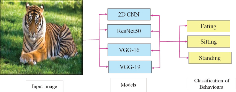
Figure 1. Block Diagram of Animal Behaviour Classification
3.1. 2D-CNN Architecture
The detailed description of each layer is given as:
1) Input layer
An input layer, an output layer, and a large number of hidden layers make up a convolutional neural network. Image and video recognition, image classification, medical image analysis, computer vision, and natural language processing are applications of CNN. The colour image has 3 (RGB) colour channels, and the grayscale image depth is one. The stride refers to the number of steps in which the filter slides over the input. When the stride value is 1, the filters are moved one pixel at a time. When the stride value is 2, they move 2 pixels at a time. Padding allows to alter the size of the output. When convolution is applied to an input, the produced output size of the matrix is reduced, resulting in information loss. To avoid this, the padding concept has been implemented. Padding is done through the input volume with zeros at the border. Valid and same are two popular padding options. The same padding indicates that the output size remains the same as the input size, and valid padding means no padding is added. The convolution operation is shown in equation (1) and the feature map size is shown in equation (2) (Sowmya et al., 2023), 2D CNN architecture is shown in Figure 2 and convolution operationis shown in Figure 3.
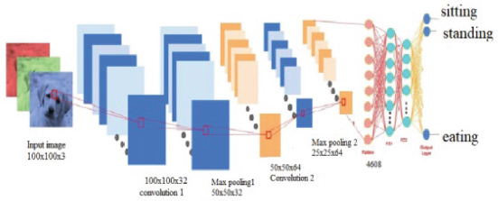
Figure 2. 2D - CNN architecture used in the proposed work (Billah et al., 2022)

Figure 3. Example of 2D CNN architecture with convolutional layer (Sowmya et al., 2023)
2) Max Pooling Layer
After convolutional layers, CNNs frequently employ the pooling layer operation (Sowmya et al., 2023). The goal is to reduce the dimension, also known as down sampling. For the pooling layer, max pooling is used which takes the maximum values from the feature map. Max Pooling is shown in equation (3) (Sowmya et al., 2023), in Figure 4.
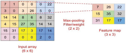
Figure 4. Example of 2D CNN architecture with Max Pooling Layer (Sowmya M et al. 2023)
In the formula, fpool represents the maximum pooling result of feature graph.
Then, features are fed into a fully connected (FC) layer which uses flattening. Flattening is used to convert all the resultant 2-dDimensional arrays from pooled feature maps into a single long continuous linear vector (Sowmya et al., 2023). Dropout and activation functions are connected to the FC layer. Dropout is used to solve the over fitting problem and improve the generalization error. An activation function decides whether a neuron should be activated or not. It helps to normalize the output of each neuron to a range between 1 and 0. The activation function used in 2D-CNN are the rectified linear unit ReLU, Softmax, tanH and the Sigmoid functions. The ReLU activation function is used in this work. The advantages of ReLU include the fact that it replaces negative values in the feature map by zero, moreover maximum threshold values are infinite, so there is no issue with the vanish gradient problem, the output prediction accuracy and r efficiency are maximum, speed is fast compared to other activation functions. Relu activation function is shown in equation (3) and it is shown in Figure 5:
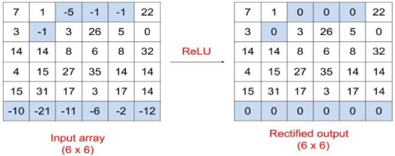
Figure 5. Example of 2D CNN architecture with Relu Activation Function (Sowmya et al., 2023)
3) Softmax Layer
Softmax is used in the last layer of a CNN to output a probability distribution over the possible classes. This is because the last layer of a CNN is responsible for making the final prediction about the class of an input image.
4) Fully Connected Layer
The fully connected (FC) layer consists of the weights and biases along with the neurons and is used to connect the neurons between two different layers. These layers are usually placed before the output layer and form the last few layers of a CNN architecture. In this, the input image from the previous layers is flattened and fed to the FC layer. The flattened vector then undergoes several more FC layers where the mathematical functions operations usually take place. In this stage, the classification process begins to take place.
Algorithm of CNN is explained as:
Algorithm of the proposed 2D CNN architecture
1: data= = []
2: labels = []
3: ListClasses = os.listdirinputDir
4: i = 0
5: for k in ListClasses do
6: Yt = np.zeros(shape = (numClasses))
7: Yt[i] = 1;
8: print(k)
9: ListFiles = os.listdir(os.path.join(inputDir, c));
10: for l in ListFiles do
11: frames = frames Extraction(os.path.join(os.path.join(inputDir, c), l))
12: end for
13: end for
14: data = np.array(data, dtype="float") / 255.0 # scale the raw pixel intensities to the range [0, 1]
Labels = np.array(labels)
15: train, testX, trainY, testY = train_test_split(X,Y)
16: model. add(Conv2D(filters = 64, kernel_size = (3, 3)))
model.add(MaxPool2D(kernel_size = (2, 2)
17: model. add (Dropout(0.25))
18: model. add (Conv2D(filters = 128, kernel_size = (3, 3)))
model.add(MaxPool2D(kernel_size = (2, 2)
model. add (Dropout(0.25))
model.add(Conv2D(filters = 256, kernel_size = (3, 3)))
model. add(MaxPool2D(kernel_size = (2, 2)
19: model.add (Dropout(0.25))
20: model.add(Flatten())
21: model.add (Dense(500))
model.add (Dense(250))
22: model.add (Dropout(0.3))
model.add(Dense(3, activation='softmax')) //3 animal behaviour classes in the output.
23: model.compile(‘adam’, loss = ‘categorical_crossentropy’, metrics = [‘accuracy’])
Pre-Processing
Before moving to image analysis, data processing is a crucial stage used to check the data values of an experiment. The image should be prepared to get an accurate result. An image resizing technique has been used in this paper. Figure 6 and Figure 7 show the resizing of images of animal behaviours.
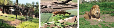
Figure 6. Original images of animal behaviours a) standing behaviour b) eating behaviour
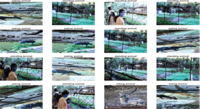
Figure 7. Resize images of animal behaviours
c) Sitting behaviour
3.2. CNN on Real Time Dataset
Four convolutional layers, four max-pooling layers, and a flattening layer are all included in a 2D CNN model. The variable number of fully connected dense layers get the flattened output as input. The first layer is made up of the unprocessed pixels from 224 x 224 animal behaviour image with three colour channels. The first convolutional layer, which has 64 filters, decreases the size to 112 x 112 x 64 by performing a dot product of the weights of the filters and the input image pixel values. To accomplish a down sampling operation, the max-pooling layer is applied along the spatial dimension (height x width), and this layer reduces the dimension to 56 x 56 x 64. Following the application of the first max-pooling layer of size 2 x 2 and output dimension of 56 x 56 x 128, the CNN filter of size 3 x 3 and with 128 filters is applied in the second layer. The output of the third layer's CNN filter, which has a 3 x 3 filtering matrix, is 28 x 28 x 256. The output of the third 2 x 2 max-pooling layer is 14 x 14 x 256. Then, in layer 5, the images are «flattened». The dense layers, which include various numbers of hidden neurons, receive these. With variable numbers of dense layers and their hidden units, several models have been created. The output layer, which is the final layer, has a softmax activation function and includes three output neurons for classification. Eating, standing and sitting categories are used for the proposed animal behaviour system.
3.3. ResNet50 Architecture
Researchers at Microsoft Research first proposed ResNet in 2015 and introduced the residual network architecture, a new design. The network's performance decreases or becomes saturated as it gets deeper. Since gradients are vanishing, accuracy is reduced. The idea of a residual network provides a solution to vanishing gradient during back propagation. Skip connections is a method used by residual networks. A skip connection links straight to the output after skipping a few stages of training. Gradients can pass directly from later levels to starting layers through the skip connections which is shown in Figure 8 (Shabir et al.,2021). Resnet is a powerful tool which is used in many computers vision tasks. It uses skip connections which adds «previous» layer output to the next layer to prevent the vanish gradient problem. It contains two blocks, namely an identity block and a convolution block. If output and input are the same then identity block is used. On the contrary if the output is not equal to the input then a convolution block is inserted to make the input e equal to the output.

Figure 8. Diagram of ResNet50 Architecture (Shabbir et al., 2021)
Skip Connection is a direct connection that skips over some layers of the model. The output is not the same due to this skip connection. Without the skip connection, input X is multiplied by the weights of the layer followed by the addition of a bias term. The activation function, F() and the output are shown in equations(5,6) (Shabbir et al., 2021) shown in Figure 9.
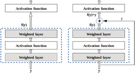
Figure 9. basic block(left) and residual block(right) of ResNet50 (He et al., 2016; Shabbir et al., 2021)
However, with the skip connection technique, the output is:
In ResNet-50, there are two kinds of blocks. One type of block is the identity block and the other one is the convolutional block.
The value of «x» is added to the output layer if and only if the
input size is equal to the output size
If this is not the case, then the «convolutional block» is added in the shortcut path to make the input size equal to the output size (Shabbir et al., 2021) which is shown in Figure 10 and Figure 11.

Figure 10. Identity block (Shabbir et al., 2021)

Figure 11. Convolution block (Shabbir et al., 2021)
There are 2 ways to make the input size equal to the output size. The first one involves padding the input volume The second one involves performing 1*1 convolutions. To equal input and output size the following equation is used It is shown in Figure 10 and Figure 11.
where, n= input image size, p=padding, s=stride, f=number of filters.
In CNNs, to reduce the size of the image, pooling is used. Resnet50, make use of stride=2 instead.
The ResNet 50 architecture contains the following elements:
Convolution with 64 distinct kernels, each with a stride of size 2, and a kernel size of 7 * 7, providing layer 1 .Next there is max pooling with also a stride size of 2.The convolution that follows has three levels: 1*1,64 kernel, 3*3,64 kernel, and finally a 1*1,256 kernel. These three layers are repeated a total of three times, yielding nine layers in this step. The kernel of “1 * 1,128” is displayed next, followed by the kernel of” 3 * 3,128” and, finally, the kernel of “1 * 1,512”. This procedure was performed four times for a total of 12 layers. Following that, we have a kernel of size 1 * 1,256, followed by two more kernels of size “3 * 3,256” and size “1 * 1,1024”; this is repeated six times, giving us a total of 18 layers. After that, a 1*1,512 kernel was added, followed by two more kernels of 3*3,512 and 1*1,2048. This process was done three times, giving us a total of «nine layers». Following that, an average pool was added and was finished with t with a layer that has three fully linked nodes, and then a Softmax function was added to give one layer.
3.4. VGG16
Figure 12 explained about VGG-16 which is trained to a deeper structure of 16 layers consisting of 13 convolution layers with five max pooling layers and three fully connected layers (Saini et al., 2023). The first two layers are convolutional layers with 3*3 filters. The first two layers contain 64 filters, resulting in a volume of 224*224*64 due to the utilization of the identical convolutions. The filters always have a 3*3 kernel size with stride value 1. This was followed by the use of a pooling layer with a max-pool of 2*2 size and stride 2, which reduces the volume&s height and width from 224*224*64 to 12*112*64.Two additional convolution layers with 128 filters are added after this. The new dimension as a result is 112*112*128.Volume is decreased to 56*56*128 once the pooling layer is employed. The size is decreased to 28*28*256 by adding two additional convolution layers, each with 256 filters. A max-pool layer separates two more stacks, each having three convolution layers. 7*7*512 volume is flattened into a fully connected (FC) layer and a softmax output of 3 classes after the last pooling layer.
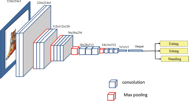
Figure 12. Architecture of VGG16 (Simonyan, K et al., 2020)
Algorithm for VGG16
Input: Videos to frames
Output: Behaviors of humans
Upload the dataset
Import required libraries
Upload train and valid path
Initialize with weights of VGG16 model.
Resize the images to fixed size 224x224.
Define Batch Size ,Image Shape
Split the dataset into training and testing.
Assign 80 % to training and 20 % to testing.
Pass the data to the dense layer.
Compile the model.
Visualize the training/validation data.
Test your model.
3.5. VGG19
VGG19 is a convolutional neural network architecture that belongs to the (Visual Geometry Group) VGG family. It was introduced in a paper entitled «Very Deep Convolutional Networks for Large-Scale Image Recognition» by Karen Simonyan and Andrew Zisserman. VGG19 is an extended version of VGG16, with 19 layers, including 16 convolutional layers and 3 fully connected layers. The architecture is known for its simplicity and uniformity, as all convolutional layers have a small receptive field (3 x 3) and a stride of 1, and the pooling layers have a 2 x 2 filter with a stride of 2. It is shown in Figure 13.
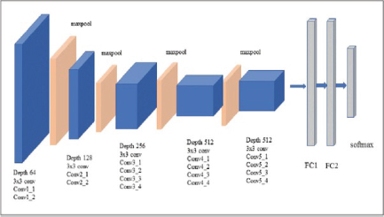
Figure 13. Architecture of VGG19(Saini et al., 2023)
Brief description of the VGG19 architecture:
Input Layer (224 x 224 x 3): Accepts input images with a size of 224 x 224 pixels and three colour channels (RGB). Convolutional layers (Conv1-Conv5). Five sets of convolutional layers, each followed by a rectified linear unit (ReLU) activation function. The convolutional layers have 64, 128, 256, 512, and 512 filters, respectively, each with a 3 x 3 kernel size and a stride of 1.
Max Pooling Layers (Pool1-Pool5): Five max pooling layers follow the convolutional blocks, each with a 2 x 2 pool size and a stride of 2. These layers progressively reduce the spatial dimensions of the feature maps.
Fully Connected Layers (FC6-FC8): Three fully connected layers follow the convolutional and pooling layers. The first two fully connected layers have 4096 neurons each, and the third fully connected layer has 3 classes
Output Layer (Softmax): The final layer uses a softmax activation function to produce probability scores for each class.
4. Experimental Results
4.1. Dataset
The dataset has been collected by using real-time videos of animals and then converting them to images. All the RGB images are fed to the CNN, VGG16 and ResNet 50 models. Training and test sets have been created from the dataset. To train the architectures, 2296 animal behaviour images were used while 575 animal behavior images were used for testing, which is shown in Table 1 and sample images is shown in Figure 13.
Table 1. Dataset Description
Behaviours |
Training Images |
Testing Images |
Eating animal |
682 |
196 |
Sitting animal |
612 |
187 |
Standing animal |
1002 |
192 |
Total |
2296 |
575 |
4.2. Performance of Animal Behaviour Classification with 2D-CNN
This section discusses the 2D-CNN training and testing method in which a real-time dataset was utilized with 8, 10, 12, and 14 layers (Indumathi et al., 2022).
As input to the model, which is displayed in Table 2, 3-dimensional input data was given along with batch size, filter size, the number of filters, the number of layers, and the number of epochs.
Table 2. 2D-CNN with 8, 10, 12, 14 layers (Indhumathi et al., 2022)
|
8 layers |
10 layers |
|
12 layers |
14 layers |
Input size |
24 x 224 x 3 |
Input size |
224 x 224 x 3 |
||
Conv 2D |
224,224,32 |
224,224,32 |
Conv 2D |
224,224,32 |
224,224,32 |
Max-pooling 2D |
112,112,32 |
112,112,32 |
Max-pooling 2D |
112,112,32 |
112,112,32 |
Conv 1 |
112,112,64 |
112,112,64 |
Conv 1 |
112,112,64 |
112,112,64 |
Max-pooling 1 |
56,56,64 |
56,56,64 |
Max-pooling 1 |
56,56,64 |
56,56,64 |
Conv 2 |
56,56,128 |
56,56,128 |
Conv 2 |
56,56,128 |
56,56,128 |
Max-pooling 2 |
28,28,128 |
28,28,128 |
Max-pooling 2 |
28,28,128 |
28,28,128 |
Conv 3 |
28,28,256 |
28,28,256 |
Conv 3 |
28,28,256 |
28,28,256 |
Max-pooling 3 |
14,14,256 |
14,14,256 |
Max-pooling 3 |
14,14,256 |
14,14,256 |
Conv 4 |
|
14,14,512 |
Conv 4 |
14,14,512 |
14,14,512 |
Max-pooling 4 |
|
7,7,512 |
Max-pooling 4 |
7,7,512 |
7,7,512 |
|
|
|
Conv 5 |
7,7,512 |
7,7,512 |
|
|
|
Max-pooling 5 |
3,3,512 |
3,3,512 |
|
|
|
Conv 6 |
3,3,512 |
|
|
|
|
Max-pooling 6 |
1,1,512 |
|
Flatten |
50176 |
25088 |
4608 |
512 |
|
Dense |
(500) |
(500) |
|
(500) |
500 |
Dense1 |
(250) |
(250) |
|
(250) |
250 |
Dense2(SoftMax) |
3 (753) |
3 (753) |
3 (753) |
3 |
|
Trainable parameters |
25,602,919 |
23,676,263 |
|
6,358,887 |
6,670,695 |
2D-CNN with 14 layers consists of 7 convolutiona layers and 7 max pooling layers. Convolutional layers 1 & 2 (112 x 112 x 64) & (56 x 56 x 128) to Maxpooling 1 & Maxpooling 2(56 x 56 x 64) & (28 x 28 x 128). Convolutionallayers 3 & 4 (28 x 28 x 256) & (14, 14, 512) to Max pooling 3 & Maxpooling 4(14 x 14 x 256) & (7 x 7 x 512). Convolutional layers 5 & 6 (7 x 7 512) & (3 x 3 x 512) to Max pooling5 & Maxpooling 6 (3 x 3 x 512) & (1 x 1 x 512.Flatten(512) parameters and dense1(500), dense2(250), SoftMax (3)outputs. Network parameters of 2D-CNN with 8 to 14 layers are given in Table 2 (Indhumathi, et al., 2022).
4.3. Performance of Animal Behaviour Classification with VGG-16
As discussed in previous sections VGG-16 is trained with 16 layers consisting of 13 convolution layers with five max pooling layers and 3 fully connected layers. The input dimension of convolutional. layer1 is 224 x 224 x 64, convolutional layer2 is 224 x 224 x 64, and Max_pooling1 is 112 x 112 x 64. The following table shows the 16 layers structure and its dimensions. Network parameters are given in the Table 3.
Table 3. Network parameters of VGG-16 (Qassim et al., 2018)
Layer (type) |
Output Shape |
Param # |
conv2d_1 (Conv20) |
(None, 224, 224, 64) |
1792 |
conv2d_2 <Conv2D) |
(None, 224, 224, 64) |
36928 |
max pooling2d_1 (MaxPooling2 |
(None, 112, 112. 64) |
0 |
conv2d_3 (Conv2D) |
(None, 112, 112, 128) |
73856 |
conv2d_4 (Conv2D) |
(None, 112, 112, 128) |
147584 |
max pooling2d_2 (HaxPooling2 |
(None, 56, 56, 128) |
0 |
conv2d_5 (Conv2D) |
(None, 56, 56, 256) |
295168 |
conv2d_6 (Conv20) |
(None, 56, 56, 256) |
590080 |
conv2d_7 (Conv2D) |
(None, 56, 56, 256) |
590080 |
max pooling2d_3 (MaxPooling2 |
(None, 23, 28, 256) |
0 |
conv2d_8 (Conv2D) |
(None, 28, 28, 512) |
1180160 |
conv2d_9 (Conv2D) |
(None, 28, 28, 512) |
2359808 |
conv2d_10 (Conv2D) |
(None, 28, 28, 512) |
2359808 |
max pooling2d_4 (HaxPooling2 |
(None, 14, 14, 512) |
0 |
conv2d_11 (Conv2D) |
(None, 14, 14, 512) |
2359808 |
conv2d_12 (Conv2D) |
(None, 14, 14, 512) |
2359808 |
conv2d_13 (Conv2D) |
(None, 14, 14, 512) |
2359808 |
max pooling2d_5 (MaxPooling2 |
(None, 7, 7, 512) |
0 |
flatten_1 (Flatten) |
(None, 25888) |
0 |
dense_1 (Dense) |
(None, 4896) |
102764544 |
dropout_1 (Dropout) |
(None, 4096) |
0 |
dense_2 (Dense) |
(None, 4096) |
16781312 |
dropout_2 (Dropout) |
(None, 4096) |
0 |
dense_3 (Dense) |
(None, 2) |
8194 |
Total params: 134,268,738
Trainable params: 134,268,738
Non-trainable params: 0
In this paper there are three behaviours, in the last layer that is in the dense layer there are 3 classes.
“FC1(Dense)” |
256 |
6422784 |
“FC2(Dense )” |
128 |
32896 |
“Softmax” |
3 |
387 |
“Trainable param” |
|
21,170,755 |
4.4. Performance of Animal Behaviour Classification with ResNet50
The back propagation method is used in this case. Convergence becomes more difficult as the network grows deeper. As discussed in previous sections ResNet-50 is trained with 50 layers. Consisting of convolutional layers with zero padding, max pooling and activation function, batch normalization layers, average pooling, and fully connected layers. The input dimension of convolutional layer1 is 224 x 224 x 64, convolutional layer2 is 224 x 224 x 64, and max_pooling1 is 55 x 55 x 64(Dar et al., 2021). Table 4 shows the 50-layer structure and its dimensions.
Table 4. Network Parameters of ResNet5 (Dar et al., 2021)
Layers |
50 Layers |
“Conv1 “ |
“7 x 7, 64, stride 2” |
|
“3 x 3 x max pool with stride 2” |
“Conv2_x” |
“[ 1 x 1,64 3 x 3,64 1 x 1,256] x 3” |
“Conv3_x” |
“[ 1 x 1,128 3 x 3,128 1 x 1,512] x 4” |
“Conv4_x” |
“[ 1 x 1,256 3 x 3,256 1 x 1, 1,1024] x 6” |
“Conv5_x” |
“[ 1 x 1,512 3 x 3,512 1 x 1,1024] x 3” |
|
Average pool |
4.5. Performance Analysis
Training and testing are an important part of any application so as to analyse the performance of the trained models. Therefore, 1984 testing samples are given to the trained model using the 2D-CNN architecture. The results predicted from the proposed model are given as confusion matrix for the classification problem. Confusion matrix is the most efficient means of identifying the true positives (TP) (Dar et al., 2022), true negatives (TN), false positives (FP), false negatives (FN) and accuracy (ACC) of a classifier, and it is used for classification problems (Wang et al., 2020) where binary or multi classes are associated with the output.
- True positive (TP): a label is predicted accurately.
- True negative (TN): the other label is predicted with accuracy.
- False positive (FP): label is predicted incorrectly.
False negative (FN): labels that are missing. The performance metrics are shown in Table 5.
Table 5. Performance metrics (Wang et al.,2020)
Performance Metrics |
Accuracy |
Precision |
Re-call |
F-score |
Formula |
||||
TP, TN, FP, FN define as True Positive, True Negative and False Positive, False Negative. |
||||
The precision and recall are combined to form a measure called F-score, which is the harmonic mean of P and R. Performance analysis for moving object detection using the proposed approach is calculated as shown in Table 5. (Wang et al., 2020; Indhumathi et al., 2022) and the performance of 2D CNN with different layers is shown in Table 6.
The performance of VGG16 and ResNet50 is shown in Table 7. Overall performance is shown in Table 8. Table 9 shows performance with existing methods.
Table 6. Comparative performance of classification of animal behaviours with real time dataset using 2D-CNN
|
2D-CNN(8 LAYERS) |
2D-CNN(10 LAYERS) |
2D-CNN(12 LAYERS) |
2D-CNN(14 LAYERS) |
||||||||
Animal Behaviors |
Precision |
Recall |
F1-score |
Precision |
Recall |
F1-score |
Precision |
Recall |
F1-score |
Precision |
Recall |
F1-score |
Eating animal |
0.99 |
0.95 |
0.97 |
0.99 |
0.94 |
0.97 |
0.72 |
0.99 |
0.84 |
0.77 |
0.99 |
0.87 |
Sitting animal |
0.88 |
0.98 |
0.93 |
0.88 |
0.93 |
0.90 |
0.99 |
0.15 |
0.26 |
0.99 |
0.08 |
0.14 |
Standing animal |
0.99 |
0.99 |
0.99 |
0.99 |
0.99 |
0.99 |
0.99 |
0.99 |
0.99 |
0.98 |
0.99 |
0.99 |
Table 7. Comparative performance of Classification of animal behaviours with real time dataset using VGG16, VGG!9 and ResNet50 (Indhumathi et al., 2022)
|
VGG16 |
VGG19 |
ResNet50 |
||||||
Animal Behaviors |
Precision |
Recall |
F1-score |
Precision |
Recall |
F1-score |
Precision |
Recall |
F1-score |
Eating animal |
0.95 |
0.92 |
0.93 |
0.94 |
0.97 |
0.96 |
0.99 |
0.99 |
0.99 |
Sitting animal |
0.74 |
0.88 |
0.80 |
0.88 |
0.91 |
0.89 |
0.99 |
0.93 |
0.97 |
Standing animal |
0.94 |
0.91 |
0.92 |
0.99 |
0.95 |
0.97 |
0.98 |
0.99 |
0.99 |
Table 8. Comparative performance of animal behaviour classification accuracy with real time dataset using 2D-CNN, VGG16 ,VGG19 and ResNet50
Model |
Accuracy |
2D-CNN |
97.73 % |
VGG16 |
91.23 % |
VGG19 |
95.45 % |
ResNet50 |
99.43 % |
The two-dimensional convolutional neural network (2D-CNN) models are tested with real time dataset and real-time video for varying numbers of convolutional layers. The 2D-CNN model that was trained with 10 convolutional layers performed well compared to 8 layers, 12 layers and 14-layer convolution models and among the three models the Resnet50 model achieved outstanding performance in comparing to the other models namely 2D-CNN, VGG19 and VGG16 which is shown in Table 8. Graphically 2D CNN with different layers is shown in Figure 15 and overall performance is shown in Figure 16.
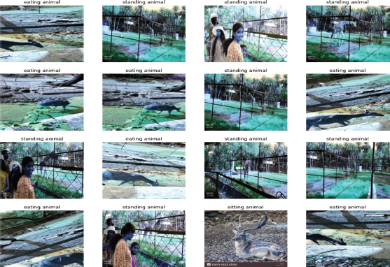
Figure 14. Sample images from real time dataset collected from zoo
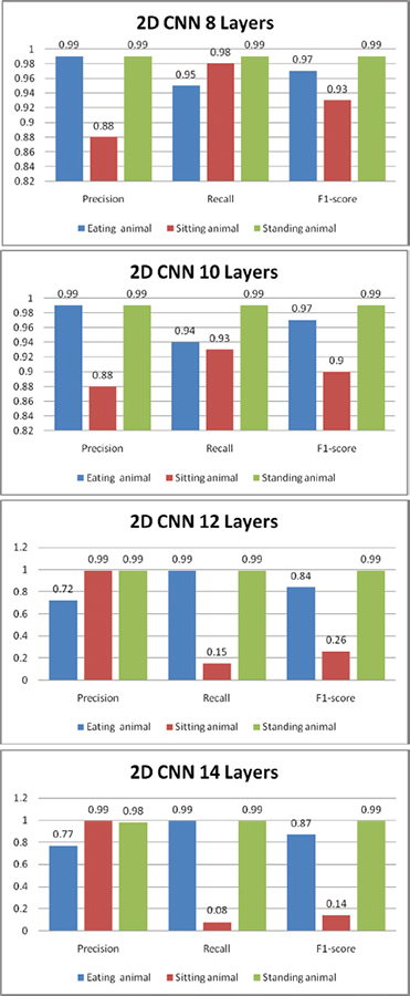
Figure 15. Overall performance of animal behaviour classification for real time dataset using 2D-CNN of a) 8Layers, b)10 Layers, c)12 Layers,d) 14 Layers using different evaluation metrics (Indhumathi, et al., 2022)
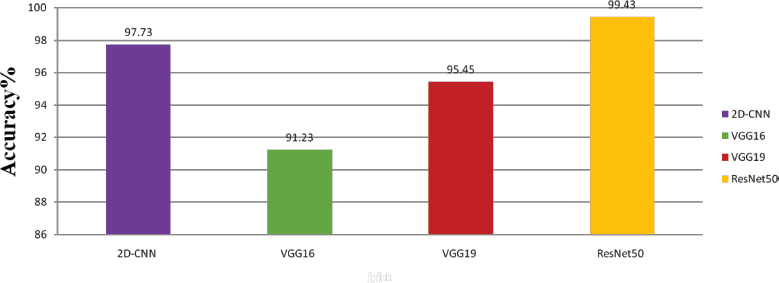
Figure 16. Overall performance of animal behaviour classification for real time dataset using VGG16 and ResNet50 of different evaluation metrics
Table 9. Comparative performance of animal behaviour in real-time video using 2D-CNN, VGG16 and ResNet50 with existing work
Existing Methods |
Methods |
Accuracy |
CNN |
93.1 % |
|
Inception-V3, SimpleRNN, LSTM, BiLSTM, and C3D on datasets for calves and cows., achieving 90.32 % and 86.67 % |
90.32 % |
|
YOLO V3 |
92.43 % |
|
Research Method |
2D-CNN |
97.73 |
|
VGG16 |
91.23 |
|
ResNet50 |
99.43 |
|
VGG19 |
95.45 |
5. Conclusion
The detection and classification of animal behaviour is an area that requires the development of effective techniques so as to reduce the problems of wildlife road accidents, which often lead to deaths and injuries. Effective classification techniques will also help farmers protect their crop yield and save their lives from dangerous animals such as elephants, tigers etc. Therefore, there is a need for a system which detects the presence of animals and gives a warning about it for security purposes. This issue can be resolved by applying CNN-based animal identification algorithms in monitoring activities, such as tracking wild animals’ movements and their travel routes in nearby forests and other areas. This would enable the forest department to take proper action and protect people and agricultural crops from animal assault. A simple CNN is a sequence of layers and mainly uses convolutional layer, a pooling layer, and a fully connected layer. Stacking these layers together creates a full convolutional neural network architecture. An algorithm has been developed and dataset images were used for the training and input images for the testing. The algorithm classifies animals efficiently with a good level of accuracy and the image of the detected animal is displayed for a better result so that it can be used for other purposes, such as detecting wild animals entering into human habitat and to prevent wildlife poaching and even human-animal conflict. A real-time dataset has been used which contains 3 classes, namely, standing, eating, and sitting. 2D-CNN, VGG16 and Resnet50 architectures were tested, out of which Resnet50 has outperformed the others, with an accuracy of 98.96 %.
References
Bhavani, D. D., Quadri, M. H. S., & Reddy, Y. R. (2019). Dog Breed Identification Using Convolutional Neural Networks on Android. CVR Journal of Science and Technology, 17(1), 62-66.
Billah, Masum, et al. «Real-time goat face recognition using convolutional neural network». Computers and Electronics in Agriculture, 194, 106730.
Bimantoro, M. Z., & Emanuel, A. W. R. (2021, April). Sheep Face Classification using Convolutional Neural Network. In 2021 3rd East Indonesia Conference on Computer and Information Technology (EIConCIT) (pp. 111-115). IEEE.
Brandes, S., Sicks, F., & Berger, A. (2021). Behaviour classification on giraffes (Giraffa camelopardalis) using machine learning algorithms on triaxial acceleration data of two commonly used GPS devices and its possible application for their management and conservation. Sensors, 21(6), 2229.
Chandrakar, R., Raja, R., & Miri, R. (2021). Animal detection based on deep convolutional neural networks with genetic segmentation. Multimedia Tools and Applications, 1-14.
Chen, G., Sun, P., & Shang, Y. (2017, November). Automatic fish classification system using deep learning. In 2017 IEEE 29th International Conference on Tools with Artificial Intelligence (ICTAI) (pp. 24-29). IEEE.
Dar, A. S., & Palanivel, S. (2022). Real-time face authentication system using stacked deep autoencoder for facial reconstruction. International Journal of Thin Film Science and Technology, 11(1), 9.
Dar, S. A., & Palanivel, S. (2021). Performance Evaluation of Convolutional Neural Networks (CNNs) And VGG on Real Time Face Recognition System. New Approaches in Commerce, Economics, Engineering, Humanities, Arts, Social Sciences and Management: Challenges and Opportunities, 143.
Debauche, O., Elmoulat, M., Mahmoudi, S., Bindelle, J., & Lebeau, F. (2021). Farm animals’ behaviors and welfare analysis with AI algorithms: A review. Revue d'Intelligence Artificielle, 35(3).
Deng, X., Yan, X., Hou, Y., Wu, H., Feng, C., Chen, L., ... & Shao, Y. (2021). DETECTION OF BEHAVIOUR AND POSTURE OF SHEEP BASED ON YOLOv3. INMATEH-Agricultural Engineering, 64(2).
Favorskaya, M., & Pakhirka, A. (2019). Animal species recognition in the wildlife based on muzzle and shape features using joint CNN. Procedia Computer Science, 159, 933-942.
Fogarty, E. S., Swain, D. L., Cronin, G. M., Moraes, L. E., & Trotter, M. (2020). Behaviour classification of extensively grazed sheep using machine learning. Computers and Electronics in Agriculture, 169, 105175.
Ghosh, P., Mustafi, S., Mukherjee, K., Dan, S., Roy, K., Mandal, S. N., & Banik, S. (2021). Image-Based Identification of Animal Breeds Using Deep Learning. In Deep Learning for Unmanned Systems (pp. 415-445).
Indhumathi, j., & balasubramanian, m. (2022). Real time video based human suspicious activity recognition using deep learning.
Manasa, K., Paschyanti, D. V., Vanama, G., Vikas, S. S., Kommineni, M., & Roshini, A. (2021, July). Wildlife surveillance using deep learning with YOLOv3 model. In 2021 6th International Conference on Communication and Electronics Systems (ICCES) (pp. 1798-1804). IEEE.
Neena, A., & Geetha, M. (2018). Image classification using an ensemble-based deep CNN. In Recent Findings in Intelligent Computing Techniques: Proceedings of the 5th ICACNI 2017, Volume 3 (pp. 445-456). Springer Singapore.
Nguyen, Hung, et al. «Animal recognition and identification with deep convolutional neural networks for automated wildlife monitoring». 2017 IEEE International Conference on Data Science and Advanced Analytics (DSAA). IEEE, 2017.
Prudhivi, L., Narayana, M., Subrahmanyam, C., Krishna, M. G., & Chavan, S. (2023, March). Animal Species Image Classification. In 2023 3rd International conference on Artificial Intelligence and Signal Processing (AISP) (pp. 1-5). IEEE..
Qassim, H., Verma, A., & Feinzimer, D. (2018, January). Compressed residual-VGG16 CNN model for big data places image recognition. In 2018 IEEE 8th annual computing and communication workshop and conference (CCWC) (pp. 169-175). IEEE
Qian, S., Ning, C., & Hu, Y. (2021, March). MobileNetV3 for image classification. In 2021 IEEE 2nd International Conference on Big Data, Artificial Intelligence and Internet of Things Engineering (ICBAIE) (pp. 490-497). IEEE.
Qiao, Y., Guo, Y., Yu, K., & He, D. (2022). C3D-ConvLSTM based cow behaviour classification using video data for precision livestock farming. Computers and Electronics in Agriculture, 193, 106650.
Sakai, K., Oishi, K., Miwa, M., Kumagai, H., & Hirooka, H. (2019). Behavior classification of goats using 9-axis multi sensors: The effect of imbalanced datasets on classification performance. Computers and Electronics in Agriculture, 166, 105027.
Schneider, S., Taylor, G. W., & Kremer, S. (2018, May). Deep learning object detection methods for ecological camera trap data. In 2018 15th Conference on computer and robot vision (CRV) (pp. 321-328). IEEE.
Shabbir, Amsa, et al. «Satellite and scene image classification based on transfer learning and fine tuning of ResNet50». Mathematical Problems in Engineering 2021 (2021): 1-18.
Simonyan, K., & Zisserman, A. (2020). Very deep convolutional networks for large-scale image recognition. arXiv 1409.1556 (09 2014). URL https://arxiv.org/abs/1409.1556. Accessed: February.
Sowmya, M., Balasubramanian, M., & Vaidehi, K. (2023). Human Behavior Classification using 2D–Convolutional Neural Network, VGG16 and ResNet50. Indian Journal of Science and Technology, 16(16), 1221-1229.
Vehkaoja, A., Somppi, S., Törnqvist, H., Cardó, A. V., Kumpulainen, P., Väätäjä, H., ... & Vainio, O. (2022). Description of movement sensor dataset for dog behavior classification. Data in Brief, 40, 107822.
Wang, H. (2020, April). Garbage recognition and classification system based on convolutional neural network VGG16. In 2020 3rd International Conference on Advanced Electronic Materials, Computers and Software Engineering (AEMCSE) (pp. 252-255). IEEE.
Wang, Xihao, Peihan Li, and Chengxi Zhu. «Classification of Wildlife Based on Transfer Learning». 2020 The 4th International Conference on Video and Image Processing. 2020.
Williams, Lauren R., et al. «Application of accelerometers to record drinking behaviour of beef cattle». Animal Production Science, 59(1), 122-132.
Wu, D., Wang, Y., Han, M., Song, L., Shang, Y., Zhang, X., & Song, H. (2021). Using a CNN-LSTM for basic behaviors detection of a single dairy cow in a complex environment. Computers and Electronics in Agriculture, 182, 106016.
Yang, Qiumei, and Deqin Xiao. «A review of video-based pig behavior recognition». Applied Animal Behaviour Science, 233, 105146.
Yudin, D., Sotnikov, A., & Krishtopik, A. (2019). Detection of big animals on images with road scenes using deep learning. In 2019 International Conference on Artificial Intelligence: Applications and Innovations (IC-AIAI) (pp. 100-1003). IEEE.
Zeng, P. (2021, December). Research on similar animal classification based on CNN algorithm. In Journal of Physics: Conference Series (Vol. 2132, No. 1, p. 012001). IOP Publishing.