ADCAIJ: Advances in Distributed Computing and Artificial Intelligence Journal
Regular Issue, Vol. 13 (2024), e31616
eISSN: 2255-2863
DOI: https://doi.org/10.14201/adcaij.31616
Optimized Deep Belief Network for Efficient Fault Detection in Induction Motor
Pradeep Kattaa, K. Karunanithia, S. P. Rajab, S. Ramesha, S. Vinoth John Prakasha, and Deepthi Josephc
a School of Electrical and Communication Engineering, Vel Tech Rangarajan Dr.Sagunthala R&D Institute of Science and Technology, Chennai, Tamilnadu, India
b School of Computer Science and Engineering, Vellore Institute of Technology, Vellore, Tamilnadu, India
c Department of Electrical and Electronics Engineering, Vel Tech Multi Tech Dr. Rangarajan Dr. Sakunthala Engineering College, Chennai, Tamilnadu, India
pradeep.2048@gmail.com, k.karunanithiklu@gmail.com, avemariaraja@gmail.com, rameshsme@gmail.com, vjp.tiglfg@gmail.com, deepths@gmail.com
ABSTRACT
Numerous industrial applications depend heavily on induction motors and their malfunction causes considerable financial losses. Induction motors in industrial processes have recently expanded dramatically in size, and complexity of defect identification and diagnostics for such systems has increased as well. As a result, research has concentrated on developing novel methods for the quick and accurate identification of induction motor problems.In response to these needs, this paper provides an optimised algorithm for analysing the performance of an induction motor. To analyse the operation of induction motors, an enhanced methodology on Deep Belief Networks (DBN) is introduced for recovering properties from the sensor identified vibration signals. Restricted Boltzmann Machine (RBM) is stacked utilizing multiple units of DBN model, which is then trained adopting Ant colony algorithm.An innovative method of feature extraction for autonomous fault analysis in manufacturing is provided by experimental investigations utilising vibration signals and overall accuracy of 99.8% is obtained, which therefore confirms the efficiency of DBN architecture for features extraction.
KEYWORDS
Induction Motor; Deep Learning; Deep Belief Networks (DBN); Restricted Boltzmann Machine (RBN); Ant Colony Algorithm
1. Introduction
Electric induction motors are perhaps the most influential component and driver of modern life in terms of production. Moreover, induction motors are extensively used within diverse industries owing to its ruggedness and robustness and requires typically low maintenance and have competitive costing (Liang et al., 2019). Induction motors are known for their robust construction and reliability. They have a simple design with fewer moving parts, which reduces the chances of mechanical failure and increases their overall durability. This makes them suitable for continuous operation in harsh environments. The high efficiency of modern induction motors facilitates the conversion of a large portion of electrical energy into mechanical energy. This energy efficiency helps in reducing power consumption and operational costs. Moreover, its simple design reduces the maintenance requirements and operational downtime, leading to lower maintenance costs over the motor’s lifespan (Le Roux and Ngwenyama, 2022; Zahraoui et al., 2022; Chang et al., 2023).
Extensive attention has been directed towards the diagnosis of faults in induction motors due to the significant economic and technical implications of unexpected downtime resulting from failures. Similar to other electrical devices, induction motors are susceptible to various types of failures. Excessive vibrations, imbalanced line currents and voltages, torque pulsations, reduced average torque, and higher heating are all symptoms of these issues. These issues further exacerbate efficiency losses in any given process (Martinez-Herrera et al., 2022), (Benninger et al., 2023). In earlier days, defect detection for induction motors was mostly based on monitoring current and vibration levels. Simple methods such as over current, over voltage, and earth-fault were commonly employed. However, with advancements in technology, a combination of traditional and modern approaches has emerged, leading to more efficient techniques for detecting faults in induction motors (Kumar and Hati, 2021). While the afore mentioned methods and techniques are effective in detecting and diagnosing individual faults in induction motors, many of them rely on complex mathematical foundations. These approaches often necessitate specialized hardware and software to convert time domain signals into frequency domain and vice versa.
A novel approach utilizing fuzzy logic technique has been suggested in (Talhaoui et al., 2022) for diagnosing broken rotor bars in an induction machine. By employing wavelet packet decomposition, this method enables the detection, identification, and prediction of faults under various operational conditions of the machine. Upon investigation, it has been observed that a substantial increase in the number of fuzzy rules leads to notable computational and interaction delays. The research in (Misra et al., 2022) introduces an effective approach to employ time frequency based feature extraction on signals captured by multiple sensors. This method enhances the information available for learning purposes, utilizing fine-tuned transfer learning models. However, the extraction of limited redefined features is only possible with this approach. In (Namdar et al., 2022), an algorithm is introduced for detecting faults by utilizing the Kalman Filter. The algorithm focuses on extracting motor current signatures and motor voltage signatures using Kalman Filter. Anyway, it did not adequately address the computational complexity and real-time implementation challenges. The work in (Kavitha et al., 2022) utilizes a giant magneto resistance broken rotor method to diagnose faults in the induction motor by analyzing an outward magnetic flux generated by the motor, enabling early-stage fault detection. However, the impacts of feasibility and practicality of the approach are not discussed. A novel fault diagnostic system utilizing infrared thermography has been introduced in (Choudhary et al., 2020), capable of automatically detecting mechanical faults in rotary machinery with exceptional precision. One potential drawback could be the reliance on a limited dataset or lack of diversity in bearing fault types, which may limit the generalizability and robustness of the proposed machine learning model. The work in (Agah et al., 2022) proposes a hybrid approach for identifying broken rotor bar and rotor mixed eccentricity faults in three-phase squirrel cage induction motors. The proposed method utilizes a single phase of the stator current signal for fault detection but exhibits limited evaluation of the proposed method. Although (Roy et al., 2020) uses an auto correlation based feature extraction technique to identify rolling bearing issues in induction motors, the work only evaluates a limited number of features. In (Husari and Seshadrinath, 2021) a unique two level hybrid hierarchical convolutional neural network combined with a support vector machine is developed for diagnosing incipient inter turn defects in drive-fed machines. This work fails to provide a clear view of real time implementation challenges. The study in (Zhao et al., 2020) introduces a novel algorithm for graph embedded semi-supervised deep neural networks. The objective functions are restructured within the framework of semi-supervised learning. However, it is worth noting that the category distribution of real industrial data often exhibits imbalances. For bearing fault diagnostics, (Toma et al., 2020) proposes a hybrid motor current data driven technique. The method employs statistical features, genetic algorithms, and machine learning models. However, comparable results are achieved solely by employing statistical features. To improve fault diagnosis and performance of classification, a study is presented in (Shi and Zhang, 2020) involving a modification approach utilizing an under sampling procedure, and a threshold adjustment using the Grey Wolf Optimizer (GWO) algorithm. Additionally, the paper did not extensively address the computational complexity. In (Hussain et al., 2022) a novel hybrid model using Matching Pursuit and Discrete Wavelet Transform is developed for fault classification by utilizing collected signals. The proposed approach incorporates an optimal feature selection mechanism and machine learning classifiers. The approach entails extracting just statistical information from the raw signal. (Lopez-Gutierrez et al., 2022) introduces a method for identifying bearing defects in an induction motor using the empirical wavelet transform, a signal processing method that decomposes the vibration signal into several components. Anyway, the impacts of the practicality of the proposed transform are not analysed.
The aforementioned shortcomings insist the need for improved diagnostic approaches for fault detection in induction motors in order to address recent challenges including complex mathematical procedures, need for specialized component setup, lack of generalizability and robustness. Hence This study suggests an efficient diagnosis technique for induction motors that makes use of deep learning to automatically recognise the functioning status and learn features from sensor data with the aid of Ant Colony optimization.
2. Proposed System
The effectiveness of fault recognition is strongly impacted by feature extraction from original signals, making it a crucial step in conventional fault detection of induction motors. Figure 1 demonstrates a DBN based method for diagnosing induction motor faults that involves building a DBN model to extract various levels of information from a training dataset.
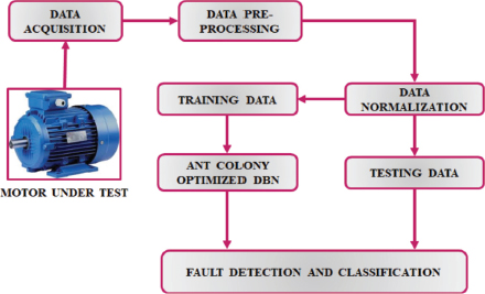
Figure 1. Proposed System Architecture
Vibration signals are adopted as input as they provide beneficial information that represents functioning status of induction motors. These signals are indicative of whether the motors are functioning correctly or if there are issues that need to be detected. The input parameters of architecture, includes a set of neuron, hidden layer, and training epochs, will first be initialised. These parameters are set up initially before the training process begins. An output of lower layer RBM is employed as training input for succeeding layer once each layer of architecture has been trained as an RBM unit.Synaptic weights and biases are established after learning of each layer, and the fundamental structure is established. Classification is a direct fine tuning process, and the suggested technique employs labelled data for training to achieve fine tuning, which enhances the discriminative performance for classification task. This fine-tuning process involves using labelled data, which means the data is tagged with the correct categories or classes. One RBM at a time is trained using an unsupervised training procedure, and the weights of the entire model are then adjusted using supervised finetuning using labels. Training error is defined as the discrepancy between target label and DBN outputs. This error helps in assessing how well the network is performing during training. Deep network parameters changes based on Ant colony optimization results in attaining minimum error. After DBN model is trained, all DBN parameters are fixed, subsequently adjacent step is to test model’s capacity for classification. The classification rate, which represents how accurately the DBN can assign data points to their correct classes or categories, is computed as a metric of evaluation.
2.1. Restricted Boltzmann Machine Model
A class of creative neural networks known as Restricted Boltzmann Machine (RBM) is capable of learning a probability distribution over its input sets. RBMs serve as powerful feature extractors and are crucial components in DBNs because they help the network learn increasingly abstract and hierarchical representations of data. These learned representations can capture meaningful features and patterns in the input data, making DBNs effective for a wide range of machine learning tasks, including image recognition, natural language processing, and more. An RBM comprises of a hidden layer where data are learned and an input layer with input as data. The RBM is a two-layer probabilistic network and a subtype of Boltzmann machine that is referred to be “restricted” since nodes in same layer is linked by each other. By recreating input, the RBM technique automatically identify patterns in data. Figure 2 illustrates the RBM’s structure.
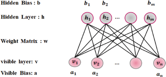
Figure 2. RBM Structure
A RBM is an energy-based system with hidden and visible nodes that have binary-type units with values between 0 and 1. The weight matrix is indicated as w = (wij)m×n, in which specifies the entry wij with weight connected to visible unit vi and hidden unit hj with corresponding bias weight as ai and bj. An energy function is used to represent the marginal distribution of a particular joint configuration (h, v):
In matrix notation it becomes:
The offset factor is specified as a = (a1, a2,…, an) for visible layer as v = (v1, v2,…, vm) and the bias vector is represented as b = (b1, b2,…, bn) for hidden layer h = (h1, h2,…, hm). Similarly, the RBM parameters to be learned is specified as θ = (a,b,w), with constants n and m indicating number of units in visible and hidden layer.
The normalization factor is given by
The joint probability distribution over the hidden or visible layers is described by the energy function as follows:
The summing of all hidden units yields probability of a visible layer, often known as training data:
Using Equation (4) log likelihood probability is written as
The following approaches for log-likelihood evaluation is utilized to solve the model parameters:
Where Ed specifies expectation under distributions defined by model, and Em indicates expectation under distribution across training data.
Since there is no connectivity across neurons in a given layer in an RBM, the expectation of data stochastic process may be estimated with ease. The likelihood that a hidden node,hj will be activated by a training vector chosen at random v, is expressed as the probability that:
Where, logistic sigmoid function is specified as σ(z) = (1 + e–z)–1
Consequently, there is no direct connection established in RBM’s visible units, and the possibilities in calculating the activation probability of visible node with hidden vector is expressed as,
The derived conditional probability is compared to the threshold (v, h) to determine a criterion for evaluating the state of Boolean vectors. The definition of hj for a hidden layer is as follows:
This criteria still applies to a visible layer.
Gradient descent is required to update weights and biases based on log-likelihoods as,
In this case, η is called the learning rate. By contrast, it is not possible to compute the expectation Em. The “Contrastive Divergence” (CD) algorithm is used with Gibbs sampling method to generate sample distributions rather than estimating Em the reconstructed expectation Erof distribution. Equation 13 is utilized instead of Equation 12.
It is typical to run Gibbs sampling procedure several times to get closer to model distribution. On the other hand, performing just one repetition is also sufficient, as shown in Figure 3.
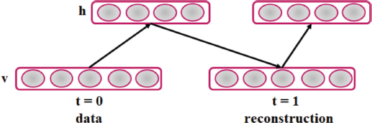
Figure 3. Representation of Single Step CD Algorithm
2.2. Architecture of DBN
Among the classes of deep neural networks, the Deep Belief Network (DBN) is a dynamic graphical model. This deep layer network is made up of multiple RBM networks that are built on top of one another. Every two consecutive hidden layers that make up a DBN architecture generate an RBM. Usually, the output previous RBM serves as input layer of the following RBM. A deep hierarchical collection of training data makes up a DBN graphical model. The following formula is used to describe joint probability distribution of visible vector v and l hidden layers (hk (k = 1, 2,…, l), h0 = v)
According to this definition, the likelihood that an inference will be made from the hidden layer hk, to visible layer v is expressed as:
Where bk is designated as kth layer bias.
In a manner similar to bottom-up inference, the top-down inference is expressed in the following symmetric form:
Where ak is designated as (k – 1)th layer bias.
Pre-training and back-propagation are the two parts of a DBN’s training process. Deep belief network training is effectively accomplished through pre-training and fine-tuning.
2.2.1. Back-Propagation of A DBN Model
After the layer-wise pretraining, backpropagation is used for supervised fine-tuning if DBN is intended for a specific supervised task like classification. Backpropagation is applied to compute gradients of the loss with respect to the network’s weights and biases, and these gradients are used to update the parameters. An unsupervised DBN architecture is then given a final layer, which represents the intended output or target, and uses back-propagation technique to accomplish supervised learning on DBN model during fine-tuning stage. The learned features in hidden layers that have been previously learned in trained RBM are refined by back-propagation method. The advantage of this method is that it employs trained weights to overcome local minimum, as opposed to typical neural network’s back-propagation, which uses random beginning weights.
2.2.2. Procedure to train DBN Model
The trained RBM’s previously learnt features are adjusted in hidden layers by back-propagation technique, and the procedure to train DBN model is depicted in Figure 4. The advantage of this method is that it employs trained weights to overcome local minimum, as opposed to typical neural network’s back-propagation, which uses random beginning weights.

Figure 4. Flowchart Representation for Training Procedure of DBN Model
2.2.2.1. Pre-Training Section
The “Greedy Layer” training technique is used to implement the pre-training segment. This method of layer-by-layer training is depicted in Figure 5. The CD technique is used to train first RBM to rebuild its inputs as accurately as feasible. An output of a second layer is introduced to operate as the visible layer of the next RBM, and so on, until the hidden layer of the first RBM is treated as the visible layer of the second RBM. This process is repeated until all predetermined hidden layers in network are trained. Prior to supervised training process, this pre-training is used to acquire the pre-trained parameters.
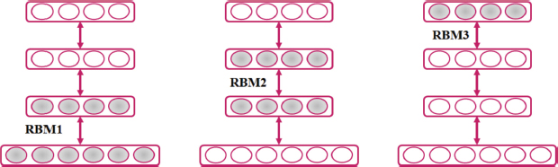
Figure 5. Layer by Layer DBN Training
2.2.2.2. Fine-Tuning Section
This phase of training is under supervision. Labelled samples are used in this stage to monitor top-down DBN model. The ideal weights and biases from each RBM’s pre-training portion are used in this section. To prevent overfitting and local optimums brought on random initialization of conventional network, the algorithms leverage the parameters acquired in training portion. Once it reaches a certain number of epochs or the goal error rate, training is terminated. As a result, the supervised learning methods improve classification performance of supervised DBN model and reduce training error.
3. Data Processing
In order to convert a raw dataset into an accessible data structure for neural network deployment, neural network models demand for a significant number of operations in preprocessing stage. The readiness of data that is appropriate for any given model determines quality of the data. Before training a models, the present neural network model handles several crucial preprocessing activities to rescale the input characteristics and target class into accessible format. Data normalization, data transformation, and data filtering or cleansing are the tasks involved. After obtaining raw data, it must first go through a rigorous cleaning procedure before being transformed and normalized. The two specially selected processing techniques that are crucial for neural network models are data transformation and data normalization. Each task’s specifics are as follows:
3.1. Data Acquisition
Data acquisition is the process of collecting and obtaining data from various sources. It is a crucial initial step in any data-driven project. The quality of the acquired data significantly influences the performance and reliability of subsequent data analysis or machine learning tasks. High-quality data is essential for accurate and reliable modelling. Data quality issues can arise due to various factors, including errors in data collection, measurement inaccuracies, inconsistencies, and missing values. Addressing these data quality issues is essential to ensure that the data is suitable for analysis and modelling. Generally, the problems with the data, such as information loss or incomprehensible values, are fixed. This implies that any anomalies, outliers, or data points that cannot be interpreted or are erroneous should be identified and rectified. Data cleaning techniques, such as outlier detection and removal, can help address these issues. Missing values in the dataset are a common data quality problem. These missing values can occur due to various reasons, including data entry errors or equipment failures during data collection.
3.2. Data Pre-Processing
In the data pre-processing phase for deep learning, it is often necessary to convert non-numeric variables into a numerical format since many deep learning architectures are designed to work with numeric data. This conversion is crucial to ensure that the model can effectively learn from and make predictions based on these variables. In the described scenario, binary and nominal characteristics, which are typically categorical in nature, are numeric-encoded. Numeric encoding assigns a unique numerical value to each category or label within these variables, enabling the model to process them. After this numeric encoding is applied, one-hot encoding is performed on the output variable. One-hot encoding is a technique used to convert categorical data into a binary format, where each category is represented as a binary vector with a “1” indicating the presence of a category and “0s” for all other categories. This process ensures that both input and output variables are in a suitable numerical format for training deep learning models while preserving the meaningful distinctions within the categorical data.
3.3. Data Normalization
In the context of neural network modeling, data normalization plays a pivotal role in addressing potential issues related to variable scales and the overall performance of the model. When input variables in a dataset have varying scales or ranges, it can lead to problems during training, especially when some variables have values in much larger or smaller magnitudes than others. Data normalization, such as min-max normalization, is employed to rescale these input characteristics to a common range, typically between 0 and 1. This rescaling process not only helps in mitigating the impact of high variance in the training data but also assists in creating a more stable and efficient training process for neural networks. By bringing all variables to a uniform scale, the model can learn more effectively, avoid issues like vanishing gradients or slow convergence, and ultimately improve its prediction performance, making it more reliable and accurate in handling a wide range of data inputs.
Following a preprocessing stage, data were divided into training and testing sets. In order to examine various sample sizes, the dataset were divided. In-order to design a reliable and efficient DBN-based model for academic assessment, optimization strategy is utilized to optimise DBN model. Here, in this work Ant Colony Optimization is used for extracting informative features and to obtain optimal results.
4. Ant Colony Optimization
An optimization method based on stochastic that mimics how actual ants behave when looking for food is called Ant Colony optimization (ACO) algorithm. Through the exchange of knowledge and cooperative effort, it determines the quickest path from an ant colony to food sources. The ants accompany one another to travel in same route. This is due to the fact that each ant, as it travels along the trail, discharges pheromones, which is a chemical substance. The other ants detect the strength of pheromone and go along where it is more concentrated. They use this strategy to locate the best route. The ants initially move about aimlessly trying to locate their objective. The ants select the road with highest pheromone concentration on their back journey based on their perception of the pheromone intensity. Because pheromone vaporises with time, the quantity of pheromone will be higher along the shortest path because the time spent travelling the shortest road will be the shortest when compared to other paths. The pheromone intensity along the shortest path would be attracted to almost every ant, making it easier for the ant to choose the path that is optimal for ants. ACO based feature extraction can provide insights into the importance and relevance of features from a large dataset. The selected features can be easily interpreted and analyzed, allowing for better understanding and insights into the underlying patterns or characteristics of the data. ACO aids in reducing dimensionality of the dataset by selecting a subset of the most discriminative features. This reduces computational complexity and enhances the performance of subsequent classification or regression tasks.
The fundamental goal of the Ant Colony Optimisation approach is to minimise the amount of redundancy between them by choosing a subset of traits that distinguish them from one another. Based on the features that have been previously selected, each ant selects a set of features that have the least similarity to those previously selected. The flowchart representation of ACO approach is illustrated in Figure 6. As a result, if one of these situations occurs, it specifies that it is the least similar to other features. The features are exposed to the most pheromone, thereby increasing the likelihood that additional ants chooses them in following iterations. Finally, because to the similarity of the traits, the major attributes selected will have high pheromone values. As a result, ACO approach selects the best features with the least amount of duplication.
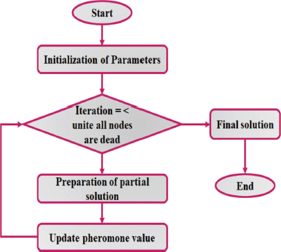
Figure 6. Flow Chart of Ant Colony Optimization
4.1. Searching Behavior
The ant in kth position, which requires to move form node i to j the following probability is utilized:
Here α and β specifies the degree of importance of pheromones and heuristic function, τij represents the concentration of pheromone between path i and j, and heuristic function equivalent to reciprocal of distance between i and j, is given by ηij.
4.2. Path Updating and Retracing
The trial values are updates after ants completing their tour is given by,
Here, the decay parameter is specified as ρ, belonging to (0, 1) to stimulate the pheromones evaporation, and ∆τij represents the total number of pheromones added by all ants.
Here, N indicates overall number of ants in nest, Q denotes pheromone update constant, the distance covered by kth ant is given by Lk and indicated the quality of pheromones added by ant k.
The following are the composition of proposed optimization strategy: Filtering out useful features using feature selection approach, optimizing the model with ideal hyper-parameter values, and regularizing network using a regularization methods. ACO helps in automating the process of hyperparameter optimization addressing the issue of generalizability. It searches the robust hyperparameter space effectively to find optimal settings, reducing the need for manual tuning thereby resulting in a more stable and reliable model that maintains consistent performance under different conditions. By leveraging the principles of swarm intelligence, ACO can discover parameter configurations that lead to improved training performance, mitigating the complexity of manual tuning. It also optimizes architectural choices for the DBN. It explores different network architectures and configurations to find setups that are well-suited to the specific problem at hand. This reduces the reliance on specialized knowledge for designing the network architecture and setup.
4.3. Feature Selection
Research in prediction and classification problems has mostly concentrated on dimensional reduction of either feature selection (FS) or feature extraction (FE) as a useful strategy for strengthening the quality of data and classification performance. The FS approach was suggested for this classification because it is the most straightforward method that successfully extracts crucial features while upholding the significance of predictive elements in dataset. One of the most well-liked FS techniques for obtaining ideal feature set is information gain (IG). Assume the characteristics A and class C, correspondingly. The entropy class C to attribute A is written by,
Here, density probability for class C is specified as P(c) An input feature’s ability to distinguish training instances according to its class label is explained by IG. The information on class C = (C1, C2,…, Cm) and m class defined the features acquired form A.
Here, En(C|A) is written as
The goal of this method is to improve performance of suggested model. The redundant, useless, and unimportant variables were eliminated. Consequently, the ideal subset of characteristics with high-quality data is found, which improves the performance of estimation techniques.
4.4. Hyperparameter Optimization
Choosing right hyperparameters for network is one of the main flaws of using DBN model. Optimising appropriate parameters will considerably boost classification performance, since it is related to reconstructing technique in CD approach of RBM training. The input data are rebuilt and reassigned to the appropriate hidden layer in every visible layer of RBM. One of the main goals of this work is to determine the effectiveness of weights and biases initiation on network output as well as robustness of proposed DBN with regard to various hyperparameters. The ability to handle challenging tasks is stronger with more complex DBN network topology. The following are the highly impacting factors taken into account in this study:
• Number of Neurons in each hidden layer
• Mini batch size
• Quantity epochs utilised in network
• Learning rate
• Number of hidden layers
• The momentum is studied throughout 0.9 to 0 and it was determined that 0.01 was an acceptable fixed value.
• A normal distribution with mean 0 and standard deviation of 0.1 is chosen in random initialization of weights.
• Initialization of the hidden and visible biases was 0.
A range of values for each hyperparameter was chosen at random in order to find the best possible structure. Until ideal values that generate best classification performance, the training is continued for randomly chosen values in range.
4.4.1. Number of Hidden Layers
Although presenting a few hidden layers is simple and inexpensive, the performance is poor. An excessive number of layers, on the other hand, will result in oversizing and expensive cost. The DBN model was practised using a specific number of hidden layers, each of which has a predetermined value to prevent complexity. However, the DBN with a single hidden layer (1L), four hidden layers (4L), and five hidden layers (5L) performed worse than the DBN with two hidden layers (2L) and three hidden layers (3L).
4.4.2. Number of Neurons in Hidden Layers
Poor performance is likely due to either too few or too many neurons (units) in each layer, similar to the amount of hidden layers. This study evaluated a range of neurons in each hidden layer to increase DBN’s performance.To determine permutations of these five values in each hidden layer, same number of 50, 100,150, 200 and 250 neurons in each hidden layer were first examined. It was discovered that the accuracy was decreased for hidden layers with values greater or lower than 50.
4.4.3. Mini Batch Size
The mini batch divides a dataset into manageable chunks and performs learning in each one. A network’s performance is strongly reliant on batch size. According to several rounds of various batch sizes, performance declines when the batch size is either too little or too large. The best batch size for datasets is between five and fifty, whereas mini-batch sizes smaller than five and greater than fifty could not yield adequate results.
4.4.4. Number of Epochs
The CD algorithm needs a specific number of iterations to settle at ideal value during each RBM training. More iterations resulted in a better result, but at the expense of greater energy consumption and over fitting during data training. The ideal epoch for pre-training phase is 20, whereas ideal epoch for fine-tuning phase is 100.
4.4.5. Learning Rate
The learning rate function successfully researched how frequently to update weights during training. A high learning rate typically speeds up training, but it does not converge or result in failure. However, training for a too-small level requires more time- and energy-intensive.
4.5. Regularization Method
Regularization is a typical technique that not only prevents overfitting but also enhances the effectiveness of neural network models.To prevent weights from becoming too enormous, the regularisation approach, also known as “Weight Decay,” is utilised in continuously to reduce weights. In neural network models, regularisation is a popular and effective strategy.The lack of weight increase is taken into consideration by adding. Weight Euclidean norm with a coefficient λ to cross entropy cost function:
The initial range of regularisation parameters was 0.01 to 0.00001, with 0.005 being an ideal fixed value.
5. Results and Discussion
Vibration signals from operational modes are present in both training dataset and testing dataset used in validating the experiment. These functioning states are simultaneously categorised using the proposed DBN-based Ant colony fault diagnosis method. The average classification is computed after 50 repetitions of each learning procedure. The training dataset in this instance contains 1200 samples, here 200 observations are considered for a single working condition whereas testing dataset includes 600 samples.
Figure 7 depicts the speed waveform of an induction motor. The motor is configured to fail, and necessary outputs are received. As a result, the power factor is calculated using RBN modelling.
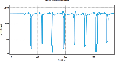
Figure 7. Waveform for motor speed
Figure 8 represents various induction motor parameters. From the figure an active current of 0.29 A is maintained constant with total current showing gradual increase from 0.25A. Correspondingly, the power factor value increases from 0.4 and reaches a unity power factor at the load.
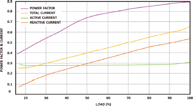
Figure 8. Parameters in induction motor
The polynomial’s coefficients are anticipated, and values of undetermined power factors are identified. This strategy offers better performance together with more adaptability and dependability. Residual errors are utilized to predict accuracy of uncertain points as shown in Figure 9. For first order the residual error of 0.02 is attained, for second order 0.00015 residual error is attained and for 3rd order residual error of 0.000020 is obtained. Therefore it is concluded that, increase polynomial order results in decreased residual error.The increase in polynomial order results in a significant decrease in residual error. In the transition from first to second order, the residual error decreased by approximately 99.25%, and in the transition from second to third order, the residual error decreased by around 86.67%.
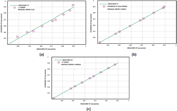
Figure 9. Residual Error (a) 1st (b)2nd and (c) 3rd Order Polynomial
Data preparation is a crucial step in classification process since raw vibration signal is constantly contaminated with noise, this noise must be removed, and the pertinent information must be extracted. With the utilization of Optimized Ant Colony Based DBN approach all the necessary features along with hyper parameters are extracted, as the output classification depends on features extracted. An improved mean square error performance of 0.01 is obtained for 200 epochs is illustrated in Figure 10. The MSE performance improves by 80% after 200 epochs of training or application. This indicates a significant enhancement in the accuracy or precision of the model or system being evaluated.

Figure 10. Training based on Optimized Ant Colony-DBN
The ROC (Receiver Operating Characteristics) Curves depicted in Figure 11, shows the performance of Classification validation and testing model. The curve is designed along True Positive Rate (TPR) and False Positive Rate (FPR). From the figure, ROC of 1 is attained during testing and validation showing excellent performance in both sensitivity and specificity. This represents a perfect classification model that achieves improved values of true positive rate and true negative rate. A good balance between sensitivity and specificity tends the proposed model to perform reliably across different datasets and applications improving the generalizability and robustness.
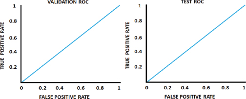
Figure 11. ROC Curves for Validating and Testing
Figure 12 illustrates the proposed Ant Colony Optimized DBN loss and accuracy. Initially, the loss is high with mild fluctuation and when the number of epochs increases a constant loss of 0.009 is maintained. Corresponding, the accuracy increases gradually and reaches a maximum accuracy of 99.8% with respect to epochs.The quantitative analysis reveals a substantial decrease in loss and a significant increase in accuracy.
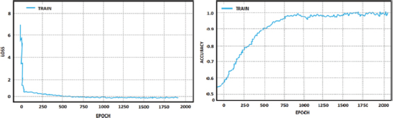
Figure 12. Training Curve for Loss and Accuracy
Table 1 demonstrates the test data classification report of Ant Colony Optimized DBN approach which effectively performs and learn features. In the table the various parameters of induction motor is given with respect to F1 score, precision, Recall and Sensitivity.
Table 1. Test dataset classification
Class |
F1-score |
Precision |
Recall |
Sensitivity |
Stator and rotor friction |
0.97 |
0.96 |
0.97 |
0.96 |
Rotor aluminium end ring break |
1.00 |
1.00 |
1.00 |
1.00 |
Poor insulation |
0.94 |
0.95 |
0.90 |
0.92 |
Bearing axis deviation |
0.95 |
0.98 |
0.97 |
0.95 |
Healthy |
1.00 |
1.00 |
1.00 |
1.00 |
Bearing noise |
0.98 |
0.95 |
1.00 |
0.98 |
Table 2 compares the performance of several techniques using parameter measurements such as MAPE, RMSE, MAE, and NAE, which stand for Mean Absolute Percentage Error, Root Mean Square Error, Mean Absolute Error, and Normalised Absolute Error, respectively. From the table, it is noted that the proposed approach results in reduced error with high advantages, when compared with the existing ones.
Table 2. Performance measure comparison
Approach |
MAPE |
RMSE |
MAE |
NAE |
DBN |
0.928 |
0.015 |
0.009 |
0.010 |
Ant Colony Optimized DBN |
0.90 |
0.011 |
0.007 |
0.005 |
SVR |
1.032 |
0.016 |
0.010 |
0.015 |
Figure 13 shows a comparison of training errors for the proposed optimised DBN and existing techniques. Form the comparison it is noted that, Ant Colony Optimized DBN functions more efficiently with reduced training error. Without optimization, the conventional DBN generates higher training error when compared to the optimized one and this significantly validates the necessity of optimization approach.It implies that the model’s performance has improved in terms of fitting the training data. A lower training error typically indicates better convergence and improved accuracy in capturing the underlying patterns and features of the dataset. A lower training error indicates that the model has successfully learned to minimize the discrepancy between its predictions and the actual training data. This suggests convergence in the optimization process and a good understanding of the training data’s patterns. This provides improved generalization ability with reliable outputs.
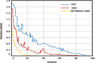
Figure 13. Training Error Comparison
Figure 14 represents the comparison graph of accuracy, in which the comparison is performed between approaches like Multi-layer perceptron (Jyothi et al., 2021), DBN (Hao et al., 2022), Hybrid SVM (Husari and Seshadrinath, 2021) and Ant Colony Optimized DBN. On comparison, the proposed optimized approach results in improved classification with accuracy of 99.8%.
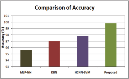
Figure 14. Comparison Graph for Accuracy
6. Conclusion
This work provides a deep learning technique based on DBN for induction motor failure prediction in manufacturing, with the frequency distribution of measured data as input. This deep architecture is constrained using Boltzmann machine as a basic block and a model built using layer-wise training. The suggested strategy makes use of DBN’s distinctive characteristics, in which the model learns numerous layers of expression and reduces training error while enhancing classification accuracy. Vibration signals are used in experiments to determine efficiency of DBN for further learning, by offering novel method of feature extraction for automated fault analysis.In contrast to conventional diagnostic techniques that require feature extraction, the proposed approach has capacity to develop hierarchical representations suited for fault classification immediately from frequency distribution of measurement data.
6.1. Conflict of Interest
The authors have no conflict of interest in publishing this work.
6.2. Plagiarism
The work described has not been published previously (except in the form of an abstract or as part of a published lecture or academic thesis), and is not under consideration for publication elsewhere. No article with the same content will be submitted for publication elsewhere while it is under review by ADCAIJ, that its publication is approved by all authors and tacitly or explicitly by the responsible authorities where the work was carried out, and that, if accepted, it will not be published elsewhere in the same form, in English or in any other language, without the written consent of the copyright-holder.
6.2. Contributors
All authors have materially participated in the research and article preparation. All authors have approved the final article to be true.
7. References
Agah, G. R., Rahideh, A., Khodadadzadeh, H., Khoshnazar, S. M. & Hedayatikia, S. (2022). Broken rotor bar and rotor eccentricity fault detection in induction motors using a combination of discrete wavelet transform and Teager-Kaiser energy operator. IEEE Transactions on Energy Conversion, 37(3), 2199-2206. https://doi.org/10.1109/TEC.2022.3162394
Benninger, M., Liebschner, M. & Kreischer, C. (2023). Fault Detection of Induction Motors with Combined Modeling-and Machine-Learning-Based Framework. Energies, 16(8), 3429. https://doi.org/10.3390/en16083429
Chang, Y., Yan, H., Huang, W., Quan, R. & Zhang, Y. (2023). A novel starting method with reactive power compensa-tion for induction motors. IET Power Electronics, 16(3), 402-412. https://doi.org/10.1049/pel2.12392
Choudhary, A., Goyal, D. & Letha, S. S. (2020). Infrared thermography-based fault diagnosis of induction motor bea-rings using machine learning. IEEE Sensors Journal, 21(2), 1727-1734. https://doi.org/10.1109/JSEN.2020.3015868
Hao, H., Fuzhou, F., Feng, J., Xun, Z., Junzhen, Z., Jun, X., Pengcheng, J., Yazhi, L., Yongchan, Q., Guanghui, S. & Caishen, C. (2022). Gear fault detection in a planetary gearbox using deep belief network. Mathematical Problems in Engineering, 2022. https://doi.org/10.1155/2022/9908074
Husari, F. & Seshadrinath, J. (2021). Incipient inter turn fault detection and severity evaluation in electric drive system using hybrid HCNN-SVM based model. IEEE Transactions on Industrial Informatics, 18(3), 1823-1832. https://doi.org/10.1109/TII.2021.3067321
Hussain, M., Memon, T. D., Hussain, I., AhmedMemon, Z. & Kumar, D. (2022). Fault Detection and Identification Using Deep Learning Algorithms in Induction Motors. CMES-Computer Modeling in Engineering Sciences, 133(2). https://doi.org/10.32604/cmes.2022.020583
Jyothi, R., Holla, T., Uma, R. K. & Jayapal, R. (2021). Machine learning based multi class fault diagnosis tool for voltage source inverter driven induction motor. International Journal of Power Electronics and Drive Systems, 12(2), 1205. https://doi.org/10.11591/ijpeds.v12.i2.pp1205-1215
Kavitha, S., Bhuvaneswari, N. S., Senthilkumar, R. & Shanker, N. R. (2022). Magnetoresistance sensor-based rotor fault detection in induction motor using non-decimated wavelet and streaming data. Automatika, 63(3), 525-541. https://doi.org/10.1080/00051144.2022.2052533
Kumar, P. & Hati, A. S. (2021). Review on machine learning algorithm based fault detection in induction motors. Archives of Computational Methods in Engineering, 28, 1929-1940. https://doi.org/10.1007/s11831-020-09446-w
Le Roux, P. F. & Ngwenyama, M. K. (2022). Static and Dynamic simulation of an induction motor using Matlab/Simulink. Energies, 15(10), 3564. https://doi.org/10.3390/en15103564
Liang, X., Ali, M. Z. & Zhang, H., 2019. Induction motors fault diagnosis using finite element method: A review. IEEE Transactions on Industry Applications, 56(2), 1205-1217. https://doi.org/10.1109/TIA.2019.2958908
Lopez-Gutierrez, R., Rangel-Magdaleno, J. D. J., Morales-Perez, C. J. & García-Perez, A. (2022). Induction machine bearing fault detection using empirical wavelet transform. Shock and Vibration, 2022. https://doi.org/10.1155/2022/6187912
Martinez-Herrera, A. L., Ferrucho-Alvarez, E. R., Ledesma-Carrillo, L. M., Mata-Chavez, R. I., Lopez-Ramirez, M. & Ca-bal-Yepez, E. (2022). Multiple fault detection in induction motors through homogeneity and kurtosis computation. Energies, 15(4), 1541. https://doi.org/10.3390/en15041541
Misra, S., Kumar, S., Sayyad, S., Bongale, A., Jadhav, P., Kotecha, K., Abraham, A. & Gabralla, L. A. (2022). Fault detection in induction motor using time domain and spectral imaging-based transfer learning approach on vibration data. Sensors, 22(21), 8210. https://doi.org/10.3390/s22218210
Namdar, A., Samet, H., Allahbakhshi, M., Tajdinian, M. & Ghanbari, T. (2022). A robust stator inter-turn fault detection in induction motor utilizing Kalman filter-based algorithm. Measurement, 187, 110181. https://doi.org/10.1016/j.measurement.2021.110181
Roy, S. S., Dey, S. & Chatterjee, S. (2020). Auto correlation aided random forest classifier-based bearing fault detection framework. IEEE Sensors Journal, 20(18), 10792-10800. https://doi.org/10.1109/JSEN.2020.2995109
Shi, Q. & Zhang, H. (2020). Fault diagnosis of an autonomous vehicle with an improved SVM algorithm subject to un-balanced datasets. IEEE Transactions on Industrial Electronics, 68(7), 6248-6256. https://doi.org/10.1109/TIE.2020.2994868
Talhaoui, H., Ameid, T., Aissa, O. & Kessal, A. (2022). Wavelet packet and fuzzy logic theory for automatic fault detec-tion in induction motor. Soft Computing, 26(21), 11935-11949. https://doi.org/10.1007/s00500-022-07028-5
Toma, R. N., Prosvirin, A. E. & Kim, J. M., 2020. Bearing fault diagnosis of induction motors using a genetic algorithm and machine learning classifiers. Sensors, 20(7), 1884. https://doi.org/10.3390/s20071884
Zahraoui, Y., Akherraz, M. & Ma’arif, A. (2022). A comparative study of nonlinear control schemes for induction motor operation improvement. International Journal of Robotics and Control Systems, 2(1), 1-17. https://doi.org/10.31763/ijrcs.v2i1.521
Zhao, X., Jia, M. & Liu, Z. (2020). Semi supervised graph convolution deep belief network for fault diagnosis of elector mechanical system with limited labeled data. IEEE Transactions on Industrial Informatics, 17(8), 5450-5460. https://doi.org/10.1109/TII.2020.3034189