
Figure 1. Fraudulent transactions significantly lower
ADCAIJ: Advances in Distributed Computing and Artificial Intelligence Journal
Regular Issue, Vol. 13 (2024), e31533
eISSN: 2255-2863
DOI: https://doi.org/10.14201/adcaij.31533
Sunil Kumar Patela and Devina Pandayb
a, b Department of Computer Science and Engineering, School of Computer Science and Engineering, Manipal University Jaipur, Jaipur, Rajasthan, India, 303007
✉ sunil.patel@jaipur.manipal.edu, devinapandeye@gmail.com
ABSTRACT
In today’s cashless society, the increasing threat of credit card fraud demands our attention. To protect our financial security, it is crucial to develop robust and accurate fraud detection systems that stay one step ahead of the fraudsters. This study dives into the realm of machine learning, evaluating the performance of various algorithms - logistic regression (LR), decision tree (DT), and random forest (RF) - in detecting credit card fraud. Taking innovation, a step further, the study introduces the integration of a genetic algorithm (GA) for feature selection and optimization alongside LR, DT, and RF models. LR achieved an accuracy of 99.89 %, DT outperformed with an accuracy of 99.936 %, and RF yielded a high accuracy of 99.932 %, whereas GA-RF (a5) achieved an accuracy of 99.98 %. Ultimately, the findings of this study fuel the development of more potent fraud detection systems within the realm of financial institutions, safeguarding the integrity of transactions and ensuring peace of mind for cardholders.
KEYWORDS
credit card fraud; logistic regression; decision tree; random forest; genetic algorithm; optimization; accuracy; precision
In today’s fast-paced world, credit cards have become essential for convenient and secure transactions, granting cardholders the power to make purchases, access cash, and defer payment within their credit limits. However, lurking in the shadows is the ever-present threat of credit card fraud, a menace that preys on unsuspecting victims. Fraudsters can swiftly exploit vulnerabilities, making unauthorized transactions and leaving cardholders in distress. As we embark on a journey toward a cashless society, it is crucial to fortify our defenses and ensure the safety of our financial transactions (Shanmugapriya et al., 2022).
As our society rapidly embraces the convenience of online payments and bids farewell to traditional cash transactions, the rise of fraud in credit cards poses a significant risk to monetary safety. Fraudsters exploit the inherent anonymity of online transactions, capitalizing on the limited information required for payment. Cardholders unknowingly fall victim to losing or stealing their sensitive data, as fraudsters clandestinely acquire card numbers, expiration dates, and CVV codes. The covert nature of these attacks leaves cardholders oblivious to the breach, only realizing their vulnerability when confronted with fraudulent purchases resulting from sophisticated phishing techniques (Harwani et al., 2020).
The application of machine learning algorithms to datasets has shown promising results in improving the accuracy of fraud detection. Various sectors, including e-commerce and banking agencies, have adopted fraud detection systems to combat the rising instances of financial fraud. With the shift from cash-based transactions to digital settlements such as debit/credit cards, online wallet payments, and online banking, the opportunities for fraudulent activities have also increased.
To tackle this growing problem against escalating issue, cutting-edge algorithms such as random forest (RF), decision tree (DT), and logistic regression (LR) have emerged as powerful allies, leveraging their predictive capabilities and pattern recognition to identify and prevent fraudulent transactions. These algorithms play a crucial role in safeguarding financial systems and protecting individuals from malicious activities aimed at personal gain (Anand and Namatherdhal, 2023).
In this study, the LR model is employed to be the preliminary model, accessing the logistic regression classifier from scikit-learn to model the probability of an event occurring. Harnessing the full potential of the training dataset, the model undergoes rigorous training. The model fearlessly ventures into uncharted territory, predicting the outcomes of the testing dataset with unmatched accuracy. The results are visualized using a heatmap and a confusion matrix, providing insights into the model’s capabilities. To further assess the model’s accuracy, metrics such as ROC AUC (Area Under the Curve) score, accuracy classification score, balanced F1 score, and precision score are calculated.
The study also introduces the decision tree model as the next approach. This model constructs a predictive model by learning decision rules derived from the data features using the decision tree classifier from scikit-learn. Just like its counterpart, the logistic regression model, the DT model is trained using the training dataset to learn the underlying patterns and relationships. Once trained, the decision tree model is applied to the test dataset, following the learned decision rules to predict the corresponding target values. The outcomes are visualized using a heatmap, and the accuracy of the model is evaluated through metrics including ROC AUC score, accuracy classification score, F1 score, and precision score (Dai, 2023).
The RF algorithm is a powerful supervised ML technique renowned for its efficacy in both classification and regression tasks. It constructs numerous decision trees on distinct subsets of the data, employing a technique known as bagging (bootstrap aggregating). Each decision tree is trained independently, utilizing a different subset of the training data through random sampling with replacement. With ensemble learning, it handles complex datasets, mitigates overfitting, and provides robustness to outliers. The algorithm captures diverse patterns and relationships, enhancing predictive accuracy and generalization (Chowdary & Kumaran, 2023).
In the initial stage, the information is gathered and stored in a sheet as a dataset. Data exploration is conducted to assess the dataset and remove any irrelevant or unnecessary data. The pre-processed data is then subjected to an RF algorithm, which is applied separately to the train and test dataset. Transaction processes can be identified as either legitimate or fraudulent through a validated analysis (Jemima et al., 2021).
To deal with high-dimensional feature spaces, we use a feature selection algorithm that combines the power of genetic algorithms and the robustness of RF as a fitness function. RF was chosen as the fitness function for GA because of its excellent performance in handling large input variable sets, automatic handling of missing values, and noise immunity. This approach allows us to pinpoint the most relevant features to our analysis without being biased by the presence of higher dimensions (Ileberi et al., 2022).
Credit card fraud detection (CCFD) is a field of data confidentiality. In this article, we present a comprehensive comparative analysis of the existing literature covering CCFD and various ML techniques used in information security. The main objective is to assess the adequacy and pertinence of distinctive ML approaches to solve complex fraud detection while maintaining the most elevated level of information security and privacy. This study aims to provide valuable insight into the most effective ML techniques to combat fraud and protect privacy by summarizing and reviewing previous research (Bin Sulaiman et al., 2022).
This study strongly contributes to the field of CCFD by examining and comparing the execution of different ML matrices calculations such as LR, DT, RF, and GA. The paper presents substantial contributions to the following areas:
• Addressing the rising threat of credit card fraud in today’s cashless society and highlighting the importance of robust fraud detection systems.
• Evaluating the performance of LR, DT, and RF algorithms in detecting fraudulent transactions.
• Introducing the use of GA with RF for feature selection, aimed at handling high-dimensional feature spaces and improving model performance.
• Comparing the effectiveness of algorithms with and without the GA feature selection.
• Providing valuable insights into the accuracy achieved by each algorithm, assisting in the development of more accurate and reliable fraud detection systems in financial institutions.
The accuracy metrics demonstrate the effectiveness, including that of GA with RF, in uncovering credit card fraud. The findings provide valuable insights for the development of more robust and accurate fraud detection systems in financial institutions.
In conclusion, this research paper aims to tackle the pressing issue of credit card fraud through the application of ML algorithms, specifically LR, DT, and RF. By leveraging these algorithms and utilizing the GA for feature selection, we strive to optimize the accuracy and effectiveness of fraud detection. Through extensive experimentation and analysis, we will compare the performance of these models and assess their suitability for detecting fraudulent transactions. The subsequent sections of this paper delve into the employed methodology, the obtained results are presented, and a comprehensive discussion of the findings is provided. Finally, we draw insightful conclusions, highlighting the strengths and limitations of the approaches explored and proposing potential lines of research in the critical domain of financial security.
In today’s rapidly evolving world of electronic commerce, the spectre of fraud looms large, wreaking havoc and inflicting substantial financial losses on a global scale. Among the various forms of fraud, credit card fraud stands out as a significant threat, impacting not only businesses but also individual clients. To combat this menace, a range of methods such as LR, RF, DT, and GA have been deployed for CCFD.
In our quest for a robust anti-fraud system, we turn to the powerful realm of artificial intelligence, specifically harnessing the capabilities of decision trees. By integrating these cutting-edge technologies through a hybrid approach, we can effectively address the challenges posed by fraudulent activities. The implementation of this innovative methodology holds the promise of substantially reducing financial losses, and safeguarding the interests of businesses and individuals alike (Shukur and Kurnaz, 2019).
The approach of Najadat et al. (2020) to detect fraudulent events is (BiLSTM) BiLSTM MaxPooling-BiGRU- MaxPooling, this approach is based on two-way long, bidirectionally gated repeat unit (BiGRU) plus short-term memory. Moreover, the authors determined 6 ML classifiers: Voting, Adaboost,RF, DT, Naive Bayes(NB) and LR. KNN achieved an accuracy of 99.13 %, LR - 96.27 %, DT - 96.40 % and NB - 96.98 %.
Tanouz et al. (2021) proposed to work with different ML-based classification algorithms - NB, LR, RF and DT - to handle strongly unbalanced data. Moreover, their study has calculations of the five units- accuracy, recall, precision, ROC-AUC curve and confusion matrix. Both LR and NB have a rating of 95.16 %, 96.77 % is the RF value and for the final model, the DT scores 91.12 %.
Alenzi & Aljehane, (2020) proposed a model to detect credit card fraud using LR, the authors achieved an all-time high score of 97.2 % in accuracy, 2.8 % error rate and 97 % sensitivity. The DT model was compared with two other classifiers, voting classifier (VC) and KNN. VC achieved 90 % accuracy, 88 % sensitivity and 10 % error, whereas KNN scored an accuracy of 93 %, sensitivity 94 % and an error rate of 7 %.
A variety of ML techniques were implemented (Tiwari et al., 2021) to detect fraudulent cases that are financially related to users but are specialized more in credit card transactions. The best ML technique used was NB, it was excellent to distinguish fraudulent transactions because it had an accuracy of 80.4 % and the area of the curve was 96.3 %.
The model given by Jain et al. (2021) incorporated various machine learning (ML) algorithms, including LR, multilayer perceptron, RF, and NB. To address the issue of dataset imbalance, the team employed the SMOTE technique for oversampling, feature selection, as well as data sharing for training and testing information. Among the evaluated models, the RF model achieved the highest score in the examination, reaching an impressive accuracy of 99.96 %. Following closely in second place was the Multilayer Perceptron model with a score of 99.93 %. The NB model came third with an accuracy of 99.23 %, while the LR model attained the lowest score at 97.46 %.
In the fight against fraud, it is imperative that we leverage the full potential of artificial intelligence and advanced algorithms to fortify our defences. By staying one step ahead of the fraudsters, we can protect the integrity of electronic transactions, foster trust in online commerce, and mitigate the devastating financial consequences caused by credit card fraud.
The methodology proposed in this research focuses on combating CCF through ML algorithms such as LR, DT, and RF. In addition, the study uses GA combined with RF for feature selection to efficiently process large features. The aim is to evaluate the performance of these algorithms in detecting fraudulent events and to compare their performance with and without GA feature selection. It highlights the study’s contribution to the growing threat of credit card fraud and provides valuable information to develop more accurate and effective fraud detection systems in financial institutions. The following sections elaborate on the methodology, present the results, and discuss the conclusions in depth.
For this study, we employed a dataset encompassing credit card transactions conducted by European cardholders during a two-day timeframe in September 2013.
The dataset comprises a total of 284,807 transactions, with a fraudulence rate of 0.172 %. It includes 30 features labelled as V1 to V28, along with Time and Amount. The dataset exclusively contains numerical attributes. The final column represents the transaction class. To ensure data security and integrity, the features V1 to V28 within the dataset are left unnamed. In this dataset, a value of 1 signifies a fraudulent transaction, while a value of 0 represents a non-fraudulent transaction (Ileberi et al., 2022).
The graph in Figure 1 visually demonstrates a notable disparity between the number of fraudulent transactions and legitimate transactions, with the former being significantly lower in count compared to the latter.
Figure 1. Fraudulent transactions significantly lower
The graph in Figure 2 illustrates the transaction amounts. It reveals a prevailing trend where the majority of transactions are relatively small in value. Conversely, only a small number of transactions approach or reach the maximum transacted amount.
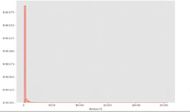
Figure 2. Concentration of small transaction amounts
The heatmap in Figure 3 displayed below provides a coloured representation of the data, allowing us to study the correlation between our predicting variables and the class variable.

Figure 3. Exploring correlations using a heatmap
In the realm of CCFD, the issue of data imbalance poses a significant challenge that researchers have diligently sought to overcome. The significant disparity in the number of genuine transactions compared to fraudulent transactions can lead to misclassification when training machine learning algorithms.
Apart from traditional under sampling and oversampling techniques, there is a popular approach called synthetic minority over-sampling technique (SMOTE). It combines the techniques of oversampling and under sampling to effectively balance the distribution of minority and majority classes in the dataset, but instead of replicating instances from the minority class, it constructs new synthetic instances using an algorithm. This helps to address the issue of imbalanced data by creating synthetic data points that resemble the minority class, thus providing a more diverse and representative training set for the machine learning algorithm.
The performance of the ML algorithm improved after applying oversampling techniques, particularly SMOTE. While it has certain drawbacks such as introducing noise and potential overlapping between classes, in the conducted experiment, SMOTE has exhibited a noteworthy advantage in terms of accuracy, surpassing other classification methods by 2- 4 % (Bin Sulaiman et al., 2022).
The SMOTE algorithm generates NM new synthetic samples for a minority class in a training set, where M represents the original number of samples for that minority class. It is crucial that N is a positive integer. In cases where N<1 is provided, the algorithm interprets the number of samples as a few classes (M=NM) and forcefully sets N=1. This can be represented by the following equation:
NM = N * M, where NM represents the number of synthetic samples generated by SMOTE, N represents the oversampling ratio or the desired number of synthetic samples per minority sample, and M represents the number of samples in the minority class as shown in Figure 4 (Meng et al., 2020).

Figure 4. Depicts the dataset after oversampling using the SMOTE algorithm
The study explores the application of advanced algorithms, such as LR, DT and RF along with GA in combating CCF. These algorithms utilize ML techniques to identify patterns and predict fraudulent transactions with remarkable accuracy. The study aims to fortify economic architectures and protect individuals from fraudulent activities, contributing to the development of more accurate and reliable CCFD systems in the financial sector as shown in Figure 7.
In constructing the classifier, logistic regression is chosen due to its advanced capabilities compared to linear regression. Unlike linear regression, logistic regression is capable of effectively categorizing data that exhibit extensive dispersion within a specified space, as illustrated in Figure 5.
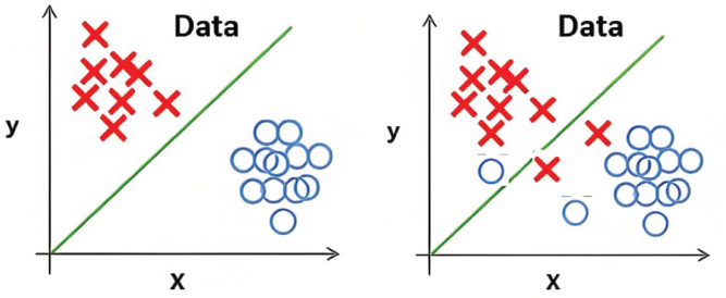
Figure 5. Precise classification with the logistic regression surpasses linear regression by effectively handling overlapping data
Linear regression, depicted on the left side, can classify data by utilizing a line to distinguish between two primary categories or classes. However, its effectiveness diminishes when data points overlap, as depicted on the right side. In such instances, linear regression fails to effectively separate the data into distinct classes. logistic regression, on the other hand, overcomes this limitation by efficiently handling overlapping data and delivering more precise classification outcomes.
Figure 6 visually compares the linear regression and logistic regression methods, emphasizing the limitation of linear regression. The purpose of this comparison is to demonstrate how logistic regression overcomes the challenge of handling overlapping data points and provides more effective classification.
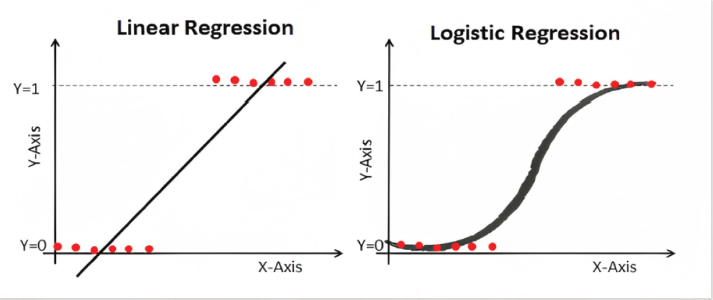
Figure 6. Logistic regression demonstrates superiority over linear regression in handling overlapping data points and achieving more accurate classification
LR offers several advantages:
1. Ease of implementation and efficiency in training: Logistic regression is simpler to implement compared to linear regression and requires less computational resources for training.
2. No assumptions about class distributions: Unlike linear regression, logistic regression does not assume any specific distribution of classes in the feature space, making it more flexible for different types of data.
3. Extension to multiple classes: Logistic regression can be easily extended to handle classification problems with multiple classes, known as multinomial regression or SoftMax regression.
4. Efficiency in classifying unknown records: Logistic regression is efficient in classifying new or unknown records once the model is trained, making it suitable for real-time applications (Alenzi & Aljehane, 2020).
The logistic regression equation can be obtained from the linear regression equation through a series of mathematical transformations:
To account for the restricted range of «t» between 0 and 1 in logistic regression, equation (1) is divided by (1 − t) as shown in equation (2):
Consequently, the logistic regression equation is defined as:
Within logistic regression, the classification task involves assigning the fraud class a value of «1» and the non-fraud class a value of «0». Typically, a threshold of 0.5 is employed to discriminate between these two classes as shown in Figure 6.
A DT is a hierarchical model that aims to divide a dataset into distinct and non-overlapping subgroups. The DT algorithm, employed in data mining, uses a recursive approach to divide the dataset into different classes through either a breadth-first or depth-first greedy method. This iterative process continues until all data items are assigned to their respective classes within the dataset. The DT structure consists of root, leaf, and internal nodes, which enable the classification of unknown data records. At every internal node, a choice is made regarding the optimal division using measures of uncertainty. The terminal nodes of the tree signify the class designations that have been allocated to the data instances (Jain et al., 2016).

Figure 7. Steps to achieve LR in CCFD
The decision tree structure shown in Figure 8 consists of roots. The decision tree algorithm offers several benefits, including its simplicity of execution, explanation, and demonstration. It is easy to understand and interpret, making it a popular choice in various domains. However, a disadvantage of this process is that it requires analysing the data step by step, which can be time-consuming for large datasets.
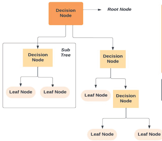
Figure 8. The structure and classification process of decision trees
When selecting the best feature for the root node and sub-nodes of a decision tree, there are two popular techniques that can be used: Attribute Selection Measures (ASM). These techniques aim to determine the most informative and discriminative features to make effective splitting decisions. The two commonly used ASM techniques (Kaul et al., 2021) are:
I. Information Gain (IG):
IG quantifies the decrease in entropy or uncertainty in the target variable (class) when a particular feature is chosen as the splitting criterion. It computes the disparity between the entropy of the parent node and the weighted average entropy of the child nodes following a split. Features that yield a higher information gain are deemed more significant for dividing the data.
Information Gain = Entropy(S)-[(Weighted Avg) * Entropy(each feature)]
II. Gini Index:
The Gini Index measures the impurity of a node by calculating the probability of misclassifying a randomly chosen element in the node. It ranges from 0 to 1, where 0 represents a completely pure node (all elements belong to the same class), and 1 represents a completely impure node (elements are evenly distributed among different classes). Features with lower Gini Index are preferred for splitting.
If P(C1|fk)> P(C2|fk) then the classififcation is C1 If P(C1|fk)< P(C2|fk) then the classififcation is C2.
The limitations of single decision trees, such as instability and sensitivity to training data, led to the development of a more robust model called random forests. RF are ensembles of regression and/or classification trees, built independently from one another. This ensemble approach shown in Figure 9 improves computational efficiency. RF introduces variance among the trees by utilizing two sources of randomness: bootstrapping the training data and selecting a random subset of attributes to build each tree. This method makes RF easy to use and enhances their predictive performance (Tiwari et al., 2021).
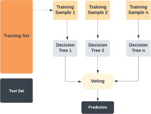
Figure 9. Enhancing predictive performance with random forests
The ensemble method used in this algorithm involves creating decision trees on the sample data and obtaining predictions from each tree. By averaging the results, this algorithm effectively reduces overfitting and improves performance compared to a single decision tree (Deepika et al., 2022) as shown in Figure 10.
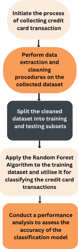
Figure 10. Steps to generate x classifiers using random forests: building trees
To produce x classifiers:
For each iteration from 1 to x, perform the following steps:
• Randomly select the training data E with replacement to generate Ej.
• Create a root node M that contains Ej and execute the function build tree (M).
• End for majority vote.
Build Tree (M): (Poojari and Joseph, 2021)
• Randomly choose x % of all potential splitting features in M.
• Identify the features F with the highest information gain for further splitting.
• Calculate the gain (N, Y) using the formula: Gain (N, Y) = Entropy (N) - Entropy (N, Y).
• To calculate the entropy, create f child nodes for each iteration from 1 to f and perform the following steps:
• Set the contents of M to Ej.
• Call the function build tree (Nj) for each child node.
• End the process.
The GA is a computational technique using heuristics for search that operates based on the principle of the survival of the fittest, inspired by natural selection [10]. The GA comprises 3 primary stages: selection, crossover, and mutation. In the selection step, the fitness of each individual in a generation is evaluated. The crossover step involves combining individuals to create new offspring. Finally, the mutation step introduces random modifications to the newly generated individuals through crossover. This process continues until the optimized solution is found, typically after numerous generations, as illustrated in Figure 11 (Chougule et al., 2015).

Figure 11. Genetic algorithm steps for evolutionary optimization
a) Unpredictably generate an initial population of chromosomes.
b) Evaluate the fitness of each chromosome using a predetermined fitness metric.
c) Choose the two parents with the greatest fitness for performing crossover or mutation operations.
d) Include a new chromosome in the succeeding generation.
e) Repeat stage c) until the size of the previous generation is equal to the next generation. Iterate stage c) until the size of the current generation matches the size of the next generation.
f) Iterate stage b) until the termination condition is satisfied.
Various techniques are utilized to select the optimal chromosomes in each iteration, such as elitism, stochastic universal selection, rank-based selection, roulette wheel selection, steady state selection, tournament selection, truncation selection, and alternative approaches. Through this selection process, the most advantageous parents are carefully chosen to generate offspring, effectively removing the less fit individuals from the population. During the crossover stage, a randomly determined crossover point is employed to exchange substrings between the parent chromosomes, producing two novel offspring. The mutation operator adds another layer of improvement to the genetic algorithm by altering specific bits within the offspring, generating new chromosomes for the subsequent population. This iterative procedure persists until all progeny have been formed (Makolo and Adeboye, 2021).
The study emphasizes the importance of gathering and storing information, conducting data exploration, and pre-processing data using ML algorithms. Results are verified to differentiate between legal and fraudulent transaction processes, visualized using a heatmap and a confusion matrix, providing insights into the model’s capabilities. Metrics such as ROC AUC score, accuracy, F1 score, and precision score are calculated to assess the model’s accuracy. It highlights the significance of addressing the rising threat of credit card fraud in today’s cashless society and emphasizes the importance of robust fraud detection systems.
Accuracy is a commonly used evaluation metric in classification tasks. It is calculated by dividing the number of accurate predictions (TP and TN) by the overall number of input samples. The accuracy can be calculated using the following:
Accuracy = (Correct Positive Predictions + Correct Negative Predictions) / (Correct Positive Predictions + Correct Negative Predictions + False Positive Predictions + False Negative Predictions)
Whereas:
• Correct Positive Prediction (CPP) implies the amount of information focuses accurately classified as positive.
• Correct Negative Prediction (CNP) implies the amount of information focuses precisely classified as negative.
• False Positive Prediction (FPP) implies the amount of information focuses inaccurately classified as positive.
• False Negative Prediction (FNP) implies the amount of information focuses inaccurately classified as negative.
As seen in Table 1, the accuracy matrix indicates a common degree of execution that shows the extent of the right predictions. That being said, in cases where the majority course outweighs the precision computation, it might not be the best appropriate measure for unequal datasets. In such cases, other assessment measurements can give a more comprehensive assessment of model performance.
Table 1. Comparing accuracy scores across different models
Accuracy Score of Various Models |
|
Logistic Regression |
0.9989993328885 |
Decision Tree |
0.999367999719109 |
Random Forest |
0.99933288859230 |
The confusion matrix is a table that summaries a model’s predicted and actual classifications on a test dataset with known true values. It gives a detailed breakdown of the model’s predictions, allowing us to assess its performance in terms of true positives (TP), true negatives (TN), false positives (FP), and false negatives (FN).
It helps us in understanding the trade-offs between false positives and false negatives and deciding the classification algorithm’s execution in recognizing card fraud. We can better understand the strengths and weaknesses of a model by examining the confusion matrix and making informed decisions about its implementation and optimization, as shown in Figures 12, 13 and 14.

Figure 12. Confusion matrix of logistic regression
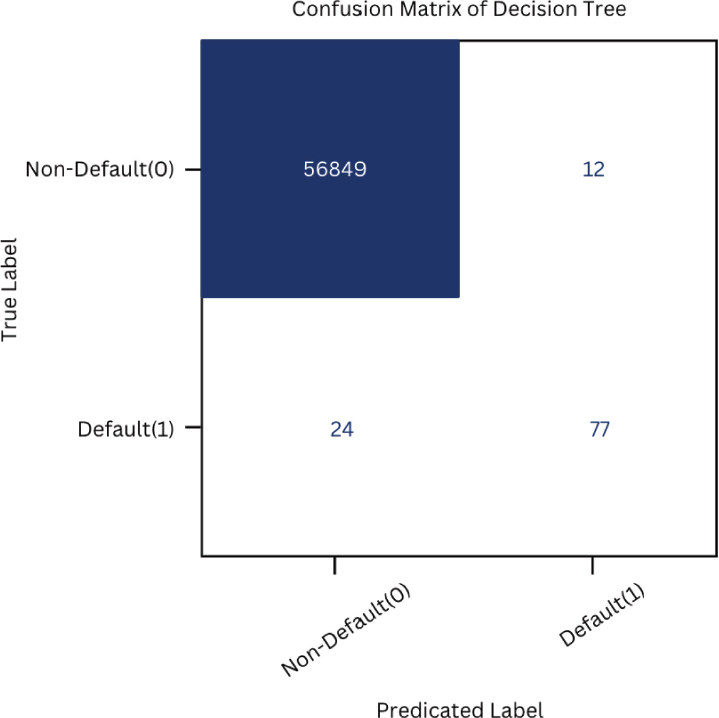
Figure 13. Confusion matrix of decision tree
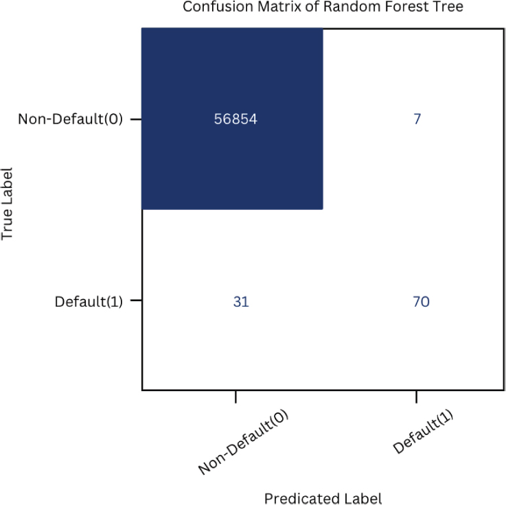
Figure 14. Confusion matrix of random forest
Positive prescient esteem (PPV) may be a metric that calculates the rate of precisely expected positive results (false exchanges) out of all anticipated positive results. It represents the classifier’s exactness in identifying false exchanges as shown in Table 2. A high precision score appears that the classifier incorporates a high wrong positive rate, suggesting that it is precise in categorising substantial exchanges as non-fraudulent.
Precision = True Positive / (True Positive + False Positive)
Table 2. Comparing precision scores across different models
Precision Score of Various Models |
|
Logistic Regression |
0.7340425531914894 |
Decision Tree |
0.8651685393258427 |
Random Forest |
0.9078947368421053 |
Recall indicates the ability of the classifier to recognize and classify all positive cases (fraud events). Recall shows the capacity of the classifier to recognize and classify all positive cases (untrue events) as shown in Table 3. A high recall rate indicates that the classifier has a low false negative rate, which means that it is able to identify most fraudulent transactions and minimize cases where the fraud is not detected.
Recall = True Positive / (True Positive + False Negative)
Table 3. Comparing recall scores across different models
Recall Score of Various Models |
|
Logistic Regression |
0.6831683168316832 |
Decision Tree |
0.7623762376237624 |
Random Forest |
0.6831683168316832 |
F1 score is a statistic that combines accuracy and recall into a single score. It is determined by taking the harmonic mean of accuracy and recall and giving equal weight to both metrics as shown as Table 4. The F1 score runs from 0 to 1, with a higher number suggesting a better balance of accuracy and memory.
Table 4. Comparing F1 scores across different models
F1 Score of Various Models |
|
Logistic Regression |
0.7076923076923077 |
Decision Tree |
0.8105263157894738 |
Random Forest |
0.7796610169491525 |
F1 Score = 2 * (Recall * Precision) / (Recall + Precision)
The classifier’s performance is determined by an overall assessment. A higher score indicates that the classifier simultaneously achieves high precision and recall, meaning that it reliably detects positive situations and minimizes false positives and false negatives.
The ROC curve illustrates how well the classification model works at various thresholds. It is a compromise between the true positive rate (TPR) and the false positive rate (FPR). TPR, also known as sensitivity or recall, assesses a classification model’s ability to properly identify positive instances. It is computed by dividing the number of TP by the sum of (TP + FN).
The FPR, also known as the false positive rate, measures the rate at which the model incorrectly classifies negative instances as positive. It is computed by dividing the number of FP by the sum of (FP + TN).
The AUC of the ROC curve quantifies the model’s capacity to discriminate between classes. It reflects the extent of distinction between the rates of true positives and false positives. A higher AUC value signifies a superior model performance, indicating a stronger capability to accurately classify instances as shown in Figures 15, 16 and 17. The AUC of the ROC curve can be used to assess how well the model differentiates between genuine transactions (0s) and fraudulent transactions (1s). A higher AUC suggests that the model is effective at correctly predicting both classes and has a good ability to distinguish between them (Marabad, 2021).
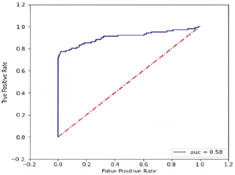
Figure 15. ROC-AUC curve of logistic regression
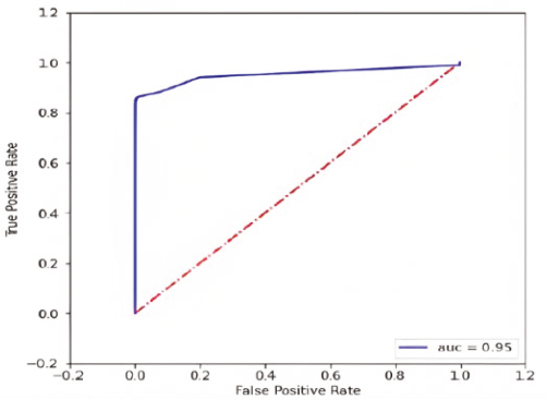
Figure 16. ROC-AUC curve of decision tree

Figure 17. ROC-AUC curve of random forest
The GA is a search algorithm that employs heuristics and operates based on the principle of «survival of the fittest» in the domain of CCFD. After applying the GA to the dataset, we obtained five feature vectors that demonstrate optimal performance. These feature vectors are labelled as a1, a2, a3, a4, and a5 as shown in Table 5. They represent the selected combinations of features that have been identified as the most effective in achieving the desired outcomes (Ileberi et al., 2022).
Table 5. Features chosen by GA
Feature Vector (a1) - |
|
Feature List for a1 |
A1, A5, A7, A8, A11, A13, A14, A15, A16, A17, A18, A19, A20, A21, A22, A23, A24, AMT |
Feature Vector (a2) - |
|
Feature List for a2 |
A1, A6, A13, A16, A17, A22, A23, A28, AMT |
Feature Vector (a3) - |
|
Feature List for a3 |
A2, A11, A12, A13, A15, A16,A17, A18, A20, A21, A24, A26, AMT |
Feature Vector (a4) - |
|
Feature List for a4 |
A2, A7, A10, A13, A15, A17, A19, A28, AMT |
Feature Vector (a5) - |
|
Feature List for a5 |
TIME, A1, A7, A8, A9, A11, A12, A14, A15, A22, A27, A28, AMT |
The initial step involves normalizing the training dataset using the min-max scaling method to ensure that all input values are within a predefined range. The primary phase entails standardizing the training dataset utilizing the min-max rescaling technique to guarantee that all input values are confined within a predetermined interval.
The feature selection component of the GA employs the GA by utilizing the standardized information from the normalize inputs module. During each stage, the GA produces a potential attribute vector (an) that is employed to train the classifiers in the training segment.
The potential attribute vector(an) is likewise utilized to evaluate the trained models with the test dataset. The evaluation procedure is performed employing the trained model component and the test data set.
Per every individual model, the testing procedure is iterated for every potential attribute vector (an) till the intended outcomes are achieved.
The overall process involves iterative normalization, feature selection, model training, and the models are optimized by employing the GA to enhance their performance in detecting credit card fraud as showcased in Table 6.
Table 6. Categorization outcomes (a1-a5)
Algorithm |
Accuracy (%) |
Precision (%) |
F1-Score (%) |
Recall (%) |
GA-RF (a1) |
99.94 |
89.69 |
82.25 |
76.99 |
GA-DT (a1) |
99.92 |
75.22 |
75.22 |
75.22 |
GA-LR (a1) |
99.91 |
82.27 |
67.70 |
57.52 |
GA-RF (a2) |
99.93 |
82.69 |
79.26 |
76.10 |
GA-DT (a2) |
99.87 |
60.62 |
64.16 |
68.14 |
GA-LR (a2) |
99.89 |
79.41 |
59.66 |
47.78 |
GA-RF (a3) |
99.94 |
85.85 |
80.18 |
75.22 |
GA-DT (a3) |
99.90 |
68.80 |
72.26 |
76.10 |
GA-LR (a3) |
99.90 |
80.00 |
63.82 |
53.09 |
GA-RF (a4) |
99.94 |
83.80 |
80.73 |
77.87 |
GA-DT (a4) |
99.91 |
75.26 |
74.13 |
76.10 |
GA-LR (a4) |
99.89 |
77.94 |
58.56 |
49.90 |
GA-RF (a5) |
99.98 |
95.34 |
82.41 |
72.56 |
GA-DT (a5) |
99.89 |
65.07 |
68.61 |
72.56 |
GA-LR (a5) |
99.77 |
34.64 |
39.84 |
46.90 |
GA-RF (an) |
87.95 |
92.63 |
84.61 |
77.87 |
GA-DT (an) |
96.91 |
71.07 |
73.50 |
76.10 |
GA-LR (an) |
93.88 |
62.96 |
61.53 |
60.17 |
To evaluate the performance of different ML models in CCFD, we calculated several key metrics as shown in the table. The table below presents the results obtained from our experiments which provide valuable insights into the performance of each enabling proactive measures against credit card fraud in today’s cashless society, as illustrated in Table 7.
Table 7. Comparative analysis of different models
Algorithm Proposed |
Accuracy (%) |
Precision (%) |
Recall (%) |
F1-score (%) |
Logistic Regression |
99.89 |
73.40 |
68.31 |
70.76 |
Decision Tree |
99.93 |
86.51 |
76.23 |
81.05 |
Random Forest |
99.93 |
90.78 |
68.31 |
77.96 |
GA-LR (a1) |
99.91 |
82.27 |
57.20 |
67.70 |
GA-DT (a1) |
99.92 |
75.22 |
75.22 |
75.22 |
GA-RF(a1) |
99.94 |
89.69 |
76.99 |
82.85 |
GA-LR (a2) |
99.89 |
79.41 |
47.78 |
59.66 |
GA-DT (a2) |
99.87 |
60.62 |
68.14 |
64.16 |
GA-RF(a2) |
99.93 |
82.69 |
76.10 |
79.26 |
GA-LR (a3) |
99.90 |
80.00 |
53.09 |
63.82 |
GA-DT (a3) |
99.90 |
68.80 |
76.10 |
72.26 |
GA-RF(a3) |
99.94 |
85.85 |
75.22 |
80.18 |
GA-LR (a4) |
99.89 |
77.94 |
46.90 |
58.56 |
GA-DT (a4) |
99.91 |
72.26 |
76.10 |
74.13 |
GA-RF(a4) |
99.94 |
83.80 |
77.87 |
80.73 |
GA-LR (a5) |
99.77 |
34.64 |
46.90 |
39.84 |
GA-DT (a5) |
99.89 |
65.07 |
72.56 |
68.61 |
GA-RF(a5) |
99.98 |
95.34 |
72.56 |
82.41 |
Our paper expands on the evaluation by including LR, DT, and RF, along with their combinations with GA. The evaluation focuses on multiple metrics, including accuracy, precision, recall, and F1-score, to provide a more nuanced understanding of algorithm performance. It demonstrates that DT outperforms the other algorithms in terms of accuracy, precision, recall, and F1-score, achieving an accuracy of 99.93 % and higher precision, recall, and F1-score compared to LR and RF, as shown in Table 8.
Analysis Table for Proposed Models - (Overview)
Table 8. Comparative analysis of various models
Algorithm |
Accuracy (%) |
Precision (%) |
Recall (%) |
F1 Score (%) |
LR |
99.89 |
73.40 |
68.31 |
70.76 |
DT |
99.93 |
86.51 |
76.23 |
81.05 |
RF |
99.93 |
90.78 |
68.31 |
77.96 |
It also shows that RF yields high accuracy (99.93 %) and maintains a good balance between precision and recall. The inclusion of the Genetic Algorithm in our paper allows for algorithm optimization. The GA is applied to feature selection and results in multiple versions (a1 to a5) of the combined algorithms (GA-LR, GA-DT, and GA-RF) as illustrated in Table 9.
Analysis Table for Proposed Models - GA
Table 9. comparison of accuracy in terms of GA (%)
Algorithm |
Baseline Model |
GA(a1) |
GA(a2) |
GA(a3) |
GA(a4) |
GA(a5) |
LR |
99.89 |
99.91 |
99.89 |
99.90 |
99.89 |
99.77 |
DT |
99.93 |
99.92 |
99.87 |
99.90 |
99.91 |
99.89 |
RF |
99.93 |
99.94 |
99.93 |
99.93 |
99.94 |
99.98 |
The existing study introduces a logistic regression-based classifier for a specific task. To prepare the data for classification, two cleaning methods are employed: the mean-based method and the clustering-based method. The classifier is then trained using the cross-validation technique with 10 folds. The results demonstrate that the LR-based classifier achieves an accuracy of 97.2 % (Alenzi & Aljehane, 2020).
However, when comparing the existing logistic regression-based classifier (referred to as the comparison model) with the proposed models’ significant improvements can be observed. The proposed base model achieves an accuracy of 99.89 %, outperforming the comparison model by a substantial margin as shown in Table 10. Furthermore, the GA-LR (a1) model, which incorporates the genetic algorithm into the logistic regression model, achieves an even higher accuracy of 99.91 % as shown in Figure 18.
LR Comparative Analysis Table – (Overview)
Table 10. Comparative analysis of logistic regression models
Model |
Accuracy (%) |
86.60 |
|
Trivedi, et al. (Trivedi et al., 2020) |
90.44 |
Suryanarayana, et al. (Suryanarayana et al., 2018) |
96.31 |
97.20 |
|
Shukur, et al. (Shukur and Kurnaz, 2019) |
97.50 |
Proposed LR Model |
99.89 |
GA-LR (a1) Model |
99.91 |
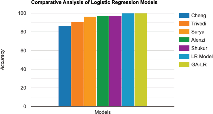
Figure 18. Visual representation of logistic regression models
The existing paper utilizes a decision tree algorithm for credit card fraud detection. The results obtained from the decision tree model show 99.98 % accuracy for real transactions. However, when it comes to fraud detection, the model has a low accuracy of 78.60 %. This shows that while the decision tree algorithm works well in identifying genuine transactions, it can be difficult to accurately detect and classify fraudulent transactions (Eswaran et al., 2021).
The benchmark model achieves a fraud detection accuracy of 78.60. On the other hand, the accuracy of the proposed basic model is significantly higher - 99.93 %, which emphasizes its superiority in accurately detecting fraudulent transactions as illustrated in Table 11. In addition, the GA-DT model (a5) outperforms the reference model with an accuracy of 99.89 % as shown in Figure 19.
DT Comparative Analysis Table – (Overview)
Table 11. Comparative analysis of decision tree models
Model |
Accuracy (%) |
Eswaran, Malathi, et al. (Eswaran et al., 2021) |
78.60 |
Hammed, et al. (Hammed, Mudasiru, and Jumoke Soyemi, 2020) |
81.60 |
Trivedi, et al. (Trivedi et al., 2020) |
90.99 |
Varun Kumar, et al. (Varun Kumar et al., 2020) |
92.88 |
Lakshmi, et al. (Lakshmi, S. V. S. S., and S. D. Kavilla, 2018) |
94.30 |
Proposed DT Model |
99.93 |
GA-DT (a5) Model |
99.89 |
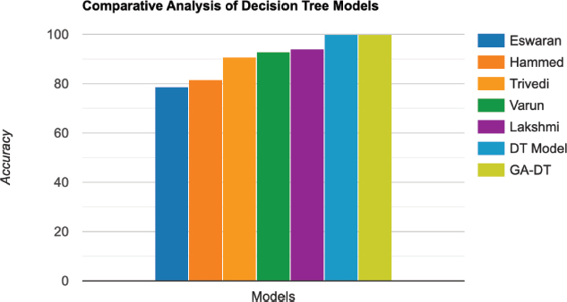
Figure 19. Visual representation of decision tree models
Existing research applies hyperparameter optimization techniques, and random forest classification (RFC) performance in CCFD. The outcome of this optimization illustrates a momentous change, with the RFC accomplishing a noteworthy precision of 98 % (Aburbeian et al., 2023).
The comparison, which is based on the RFC classifier, accomplishes a precision of 98 %. In any case, the accuracy of the suggested base model and the GA-RF (a5) show outperform that of the comparison. The proposed base model achieves an accuracy of 99.93 %, showing a significant improvement over the comparison model, as seen in Table 12. Furthermore, the GA-RF (a5) model, which incorporates the genetic algorithm for optimization, achieves an even higher accuracy of 99.98 %, as shown in Figure 20.
Comparative Analysis Table of RF –
Table 12. Comparative analysis of random forest models
Model |
Accuracy (%) |
98.00 |
|
Trivedi, et al (Trivedi et al., 2020) |
94.99 |
Shirgave, Suresh, et al. (Shirgave, Suresh, et al., 2019) |
96.20 |
More, Rashmi, et al. (More, Rashmi, et al., 2021) |
97.93 |
Niveditha, et al. (Niveditha, G., Abarna, K., and Akshaya, G. V., 2019) |
98.60 |
Proposed RF Model |
99.93 |
GA-RF (a5) Model |
99.98 |
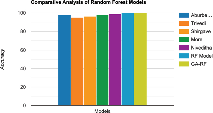
Figure 20. Visual representation of random forest models
Among the evaluated algorithms, logistic regression achieved an accuracy of 99.89 %, with precision, recall, and F1-score of 73.40 %, 68.31 %, and 70.76 %, respectively. Decision tree performed slightly better with an accuracy of 99.936 %, and higher precision, recall, and F1-score of 86.51 %, 76.23 %, and 81.05 %, respectively. Random forest also yielded high accuracy (99.932 %) with a precision of 90.78 %, recall of 68.31 %, and F1-score of 77.96 %.
The GA algorithm with different versions (a1 to a5) combined with logistic regression (GA-LR), decision tree (GA-DT), and random forest (GA-RF) showed varying performance. For example, GA-RF (a1) achieved an accuracy of 99.94 % with a precision of 89.69 %, recall of 76.99 %, and F1-score of 82.85 %. However, other versions of the GA algorithm exhibited different trade-offs regarding recall, F1-score and precision.
Based on the results, it can be concluded that DT and RF algorithms, both with and without the GA feature selection, performed well in detecting credit card fraud. They demonstrated high accuracy and relatively balanced precision and recall values. Although logistic regression achieves high accuracy, it shows lower precision and recall compared to the tree-based algorithms.
The GA algorithm, when combined with the classification models, provided an improvement in certain cases, but the performance varied depending on the specific version used. Further analysis and optimization of the GA parameters may be necessary to enhance its effectiveness for CCFD. The obtained results can be valuable for developing more robust and accurate fraud detection systems in financial institutions.
Aburbeian, A. M., & Ashqar, H. I. (2023). Credit Card Fraud Detection Using Enhanced Random Forest Classifier for Imbalanced Data. Proceedings of the 2023 International Conference on Advances in Computing Research (ACR’23). Cham: Springer Nature Switzerland. https://doi.org/10.1007/978-3-031-33743-7_48
Alenzi, H. Z., & O, N. (2020). Fraud Detection in Credit Cards using Logistic Regression. International Journal Of Advanced Computer Science And Applications, 11(12). https://doi.org/10.14569/ijacsa.2020.0111265
Anand, G., & Bharatwaja, N. (2023). An Efficient Fraudulent Activity Recognition Framework Using Decision Tree Enabled Deep Artificial Neural Network. International Research Journal of Modernization in Engineering Technology and Science (IRJETS), 5.
Bin Sulaiman, R., Schetinin, V., & Sant, P. (2022). Review of Machine Learning Approach on Credit Card Fraud Detection. Human-Centric Intelligent Systems, 2(1-2), 55-68. https://doi.org/10.1007/s44230-022-00004-0
Cheng, H. (2023). Credit Card Fraud Detection Using Logistic Regression and Machine Learning Algorithms. Diss. University of California, Los Angeles.
Chougule, P., et al. (2015). Genetic K-means algorithm for credit card fraud detection. International Journal of Computer Science and Information Technologies (IJCSIT), 6(2), 1724-1727.
Chowdary, B. Sri Sai, & Kumaran, J. C. (2023). Analytical Approach For Detection Of Credit Card Fraud Using Logistic Regression Compared With Noval Random Forest. European Chemical Bulletin, 12(1 Part-A).
Dai, M. (2023). Multiple Machine Learning Models on Credit Card Fraud Detection. BCP Business & Management, 44, 334-338. https://doi.org/10.54691/bcpbm.v44i.4839
Deepika, K., Nagenddra, M. P. S., Ganesh, M. V., & Naresh, N. (2022). Implementation of Credit Card Fraud Detection Using Random Forest Algorithm. International Journal For Research In Applied Science And Engineering Technology, 10(3), 797-804. https://doi.org/10.22214/ijraset.2022.40702
Eswaran, M., et al. (2021). Identification of Credit Card Fraud Detection Using Decision Tree and Random Forest Algorithm. International Journal of Aquatic Science, 12(3), 1646-1654.
Hammed, M., & Jumoke, S. (2020). An implementation of decision tree algorithm augmented with regression analysis for fraud detection in credit card. International Journal of Computer Science and Information Security (IJCSIS), 18(2), 79-88.
Harwani, H., et al. (2020). Credit card fraud detection technique using a hybrid approach: An amalgamation of self-organizing maps and neural networks. International Research Journal of Engineering and Technology (IRJET) 7.2020.
Ileberi, E., Sun, Y., & Wang, Z. (2022). A machine learning based credit card fraud detection using the GA algorithm for feature selection. Journal Of Big Data, 9(1). https://doi.org/10.1186/s40537-022-00573-8
Jain, R., Gour, B., & Dubey, S. (2016). A Hybrid Approach for Credit Card Fraud Detection using Rough Set and Decision Tree Technique. International Journal Of Computer Applications, 139(10), 1-6. https://doi.org/10.5120/ijca2016909325
Jain, S., Verma, N., Ahmed, R., Tayal, A., & Rathore, H. (2021). Credit Card Fraud Detection Using K-Means Combined with Supervised Learning. In Lecture notes in networks and systems (pp. 262-272). https://doi.org/10.1007/978-3-030-96305-7_25
Jemima Jebaseeli, T., Venkatesan, R., & Ramalakshmi, K. (2021). Fraud detection for credit card transactions using Random Forest algorithm. Intelligence in Big Data Technologies—Beyond the Hype: Proceedings of ICBDCC 2019. Springer Singapore. https://doi.org/10.1007/978-981-15-5285-4_18
Kaul, A., Chahabra, M., Sachdeva, P., Jain, R., & Nagrath, P. (2021). Credit card fraud detection using different ML and DL techniques. Proceedings of the International Conference on Innovative Computing & Communication (ICICC) 2021. https://doi.org/10.2139/ssrn.3747486
Lakshmi, S. V. S. S., & S. D. Kavilla. (2018). Machine learning for credit card fraud detection system. International Journal of Applied Engineering Research, 13(24), 16819-16824.
Makolo, A., & Adeboye, T. (2021). Credit card fraud Detection System using Machine learning. International Journal of Information Technology and Computer Science, 13(4), 24-37. https://doi.org/10.5815/ijitcs.2021.04.03
Marabad, S. (2021). Credit Card Fraud Detection using Machine Learning. Asian Journal For Convergence In Technology (AJCT), 7(2), 121-127. https://doi.org/10.33130/ajct.2021v07i02.023
Meng, C., Zhou, L., & Liu, B. (2020). A case study in Credit Fraud Detection with SMOTE and XGBoOST. Journal of Physics Conference Series, 1601(5). IOP Publishing. https://doi.org/10.1088/1742-6596/1601/5/052016
More, R., et al. (2021). Credit card fraud detection using supervised learning approach. Int. J. Sci. Technol. Res, 9, 216-219.
Najadat, H., et al. (2020). Credit card fraud detection based on machine and deep learning. 2020 11th International Conference on Information and Communication Systems (ICICS). IEEE, 2020. https://doi.org/10.1109/ICICS49469.2020.239524
Niveditha, G., Abarna, K., & Akshaya, G. V. (2019). Credit card fraud detection using random Forest algorithm. International Journal of Scientific Research in Computer Science Engineering and Information Technology, 301-306. https://doi.org/10.32628/cseit195261
Poojari, M., & Jobin, J. (2021). Credit Card Fraud Detection Using Random Forest Algorithm. International Journal of Trendy Research in Engineering and Technology, 5(3).
Shanmugapriya, P., Shupraja, R., & Madhumitha, V. (2022). Credit card fraud detection system using CNN. International Journal for Research in Applied Science and Engineering Technology, 10(3), 1056-1060. https://doi.org/10.22214/ijraset.2022.40799
Shirgave, S., et al. (2019). A review on credit card fraud detection using machine learning. International Journal of Scientific & technology research, 8(10), 1217-1220.
Shukur, H. A., & Sefer, K. (2019). Credit card fraud detection using machine learning methodology. International Journal of Computer Science and Mobile Computing, 8(3), 257-260.
Suryanarayana, S. V., Balaji, G. N., & Rao, G. V. (2018). Machine learning approaches for credit card fraud detection. International Journal of Engineering & Technology, 7(2), 917. https://doi.org/10.14419/ijet.v7i2.9356
Tanouz, D., et al. (2021). Credit card fraud detection using machine learning. 2021 5th International Conference on Intelligent Computing and Control Systems (ICICCS). IEEE. https://doi.org/10.1109/ICICCS51141.2021.9432308
Tiwari, P., et al. (2021). Credit card fraud detection using machine learning: a study. arXiv preprint https://doi.org/arXiv:2108.10005
Trivedi, N. K., Simaiya, S., Lilhore, U. K., & Sharma, S. K. (2020). An efficient credit card fraud detection model based on machine learning methods. International Journal of Advanced Science and Technology, 29(5), 3414-3424.
Varun Kumar, K. S., Vijaya Kumar, V. G., Vijay Shankar, A., & Pratibha, K. (2020). Credit card fraud detection using machine learning algorithms. International Journal of Engineering Research & Technology (IJERT), 9(7).