ADCAIJ: Advances in Distributed Computing and Artificial Intelligence Journal
Regular Issue, Vol. 12 N. 1 (2023), e31509
eISSN: 2255-2863
DOI: https://doi.org/10.14201/adcaij.31509
Service Chain Placement by Using an African Vulture Optimization Algorithm Based VNF in Cloud-Edge Computing
Abhishek Kumar Pandey and Sarvpal Singh
Information Technology and Computer Application, Madan Mohan Malaviya University of Technology, Gorakhpur, India-273010.
akpsiet@gmail.com, spscs@mmmut.ac.in
ABSTRACT
The use of virtual network functions (VNFs) enables the implementation of service function chains (SFCs), which is an innovative approach for delivering network services. The deployment of service chains on the actual network infrastructure and the establishment of virtual connections between VNF instances are crucial factors that significantly impact the quality of network services provided. Current research on the allocation of vital VNFs and resource constraints on the edge network has overlooked the potential benefits of employing SFCs with instance reuse. This strategy offers significant improvements in resource utilization and reduced startup time. The proposed approach demonstrates superior performance compared to existing state-of-the-art methods in maintaining inbound service chain requests, even in complex network typologies observed in real-world scenarios. We propose a novel technique called African vulture optimization algorithm for virtual network functions (AVOAVNF), which optimizes the sequential arrangement of SFCs. Extensive simulations on edge networks evaluate the AVOAVNF methodology, considering metrics such as latency, energy consumption, throughput, resource cost, and execution time. The results indicate that the proposed method outperforms BGWO, DDRL, BIP, and MILP techniques, reducing energy consumption by 8.35%, 12.23%, 29.54%, and 52.29%, respectively.
KEYWORDS
cloud-edge network; VNF; AVOA; service function chain; physical network
1. Introduction
Cloud-edge computing is positioned between end-user devices and service providers. The technology facilitates the computation of vast quantities of information at the network’s edge. This leads to enhanced adaptability and mobility in the underlying network infrastructure. The primary goal of the computing facility in edge computing is to reduce the load on the primary network connections and alleviate end-to-end customer congestion. However, the notable reliance on specialized technology presents a significant obstacle to the progression of cloud-edge computing. Virtual network functions (VNF) have been advocated by service providers as a means of enabling more flexible service delivery in the edge network. Network function virtualization (NFV) enables the transformation of unwieldy hardware middleboxes, including firewalls, encryption, and load balancers, into virtualized network functions (VNFs) that are executed using lightweight software. Virtualized network functions (VNFs) can be deployed within a virtualized infrastructure, such as a containerized environment (Cziva et al., 2017; Attaoui et al., 2022). Through the deployment of virtual network function (VNF) instances in peripheral networks, service providers can achieve enhanced service delivery and scalability, while also optimizing their financial performance by reducing both operating expenditures and capital expenditures. The concatenation of multiple Virtual Network Functions (VNFs) can lead to the creation of intricate services. Furthermore, virtualization techniques are employed with the aim of enhancing the overall programmability and adaptability of the cloud-edge network. Service function chaining (SFC) is a technique that is noteworthy, as it ensures the proper handling and chaining of virtualized instances (Almurshed et al. 2022; Khan et al., 2019; Abbas et al., 2017). This is achieved through the utilization of a manager module, which guarantees the appropriate synchronization of chain placement. Furthermore, it is accountable for overseeing the complete lifecycle of virtual network functions (VNFs), encompassing the initiation, expansion, and modification of network functions (Ale et al., 2021).
The initiative of network function virtualization aims to separate network software from the utilization of specialized, proprietary hardware components, commonly referred to as "middleboxes" (such as traffic shapers and network address translation boxes). Likewise, the utilization of application virtualization enables an application to function within an isolated virtualized setting (Matias et al., 2015). In the context of cloud-based or service-based application architectures, it is common for an application to consist of numerous components, with each component functioning as a virtual function (VF).
In the realm of application service virtualization, multiple virtual functions (VFs) have the capability to function on a generic computing device through a virtual machine, operating system container, or serverless environment (Schardong et al., 2021). The adaptability of virtual machines in terms of deployment, management, resource allocation, and migration enable their hosting in proximity to users, either in an edge cloud or data centre, to satisfy the application’s demands for high throughput and ultra-low latency (Gao et al., 2022). The network depicted in Fig. 1 comprises 8 nodes and 11 links. Physical nodes known as edge servers are deployed by a remote cloud orchestrator to facilitate the deployment of SFCs.
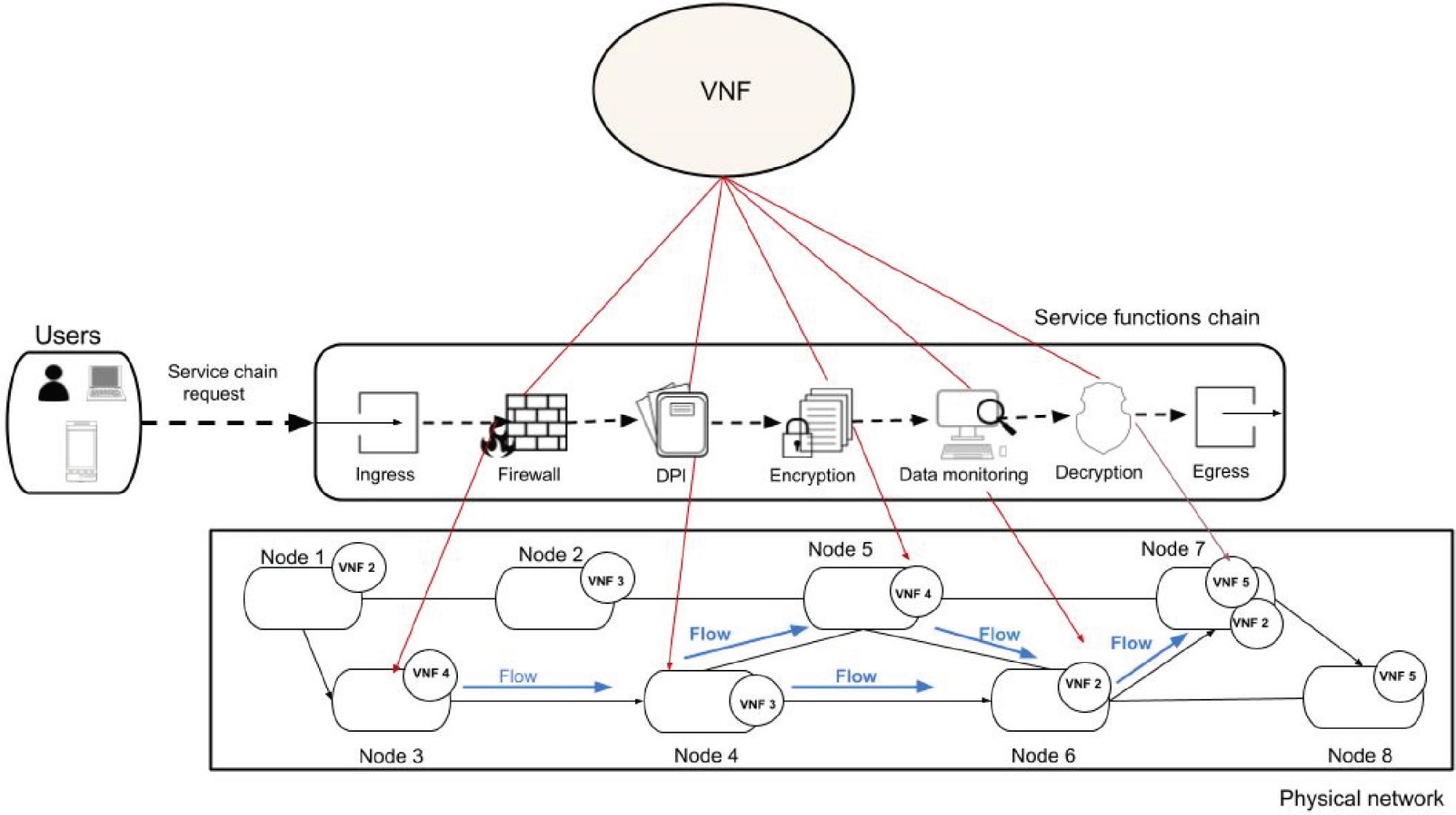
Figure 1. An architecture of an SFC deployment
African vulture optimization has been used in a broad variety of experiments to successfully handle the SFC placement problem (Abdollahzadeh et al., 2021). AVOA is able to identify appropriate locations for the deployment of VNFs in different situations, and it is consistent with the changing environment. In this article, we present an AVOA-based dynamic SFC placement technique with parallelized VNFs that aims to optimize the long-term estimated cumulative dividend. This method works with parallelized VNFs. The integer linear programming (ILP) solution to the SFC placement problem in distributed networks is a novel strategy that makes use of an algorithm. The proposed method is able to accomplish computational acceleration in the process of delivering online services because of its ability to share VNFs in parallel for SFCs. In addition, proposed method contains a strategy for extracting the distribution of initialized VNFs, which, if implemented, has the potential to increase the acceptance rate of subsequent requests (Tomaselli et al., 2018).
Through the configuration of a VNF queue network, this approach has the ability to anticipate which action will be the most appropriate for actors working in SFC placement (Tajiki et al., 2018).
The major contribution of this article is as follows:
• To determine VNF placement is a multi-objective optimization issue that minimizes edge node delay cost, energy consumption, total delay cost, resource cost, throughput, and execution time of the cloud-edge network.
• The proposed model incorporates virtual service networks, which will allow it to meet the needs of future applications in the edge network. The needs of outlying networks are met by these systems.
• The findings from a comprehensive evaluation reveal several benefits of managing virtual service networks in comparison to the state-of-the-art methods.
• The proposed method has thoroughly outperformed existing methods such as BGWO (Shahjalal et al., 2022), DDRL (Khoshkholghi et al., 2022), BIP (Akhtar et al., 2021), and MILP (Magoula et al., 2021) when compared to state-of-the-art optimized algorithms based on AVOA.
The rest of the manuscript is given as follows. In section 2, related work is presented, system model and problem formulation and proposed work i.e., AVOAVNF, are discussed in Section 3 and Section 4. Further, in Section 5, we discuss the simulation results. Finally, the conclusion is given in Section 6.
2. Literature Review
This section provides a summary of the present computational application situations that necessitate the use of edge computing platforms, in addition to a discussion of the essential elements that assist edge computing in providing SFC and VNF services. The service chain refers to the requirement that the request from the end user must be performed by numerous services that are dependent on one another. The management of service chain positioning receives a new facet with the addition of inter-service interdependence. For example, the end-to-end latency of a user request throughout the service chain ought to incorporate the communication latency that exists between the contingent services and the movement of traffic. It may be possible to loosen some restrictions to facilitate the development of solutions that are better suited to handle the complications of service chain positioning (Shahjalal et al., 2022; Wang et al., 2017).
Wang et al. (2019) focused on the positioning of service chains in MEC in order to evenly distribute the activity across the nodes. The writers modelled each service network as its own graph, with each vertex and line corresponding to a different service or communication route. The subsequent distribution challenge is an NP-hard one, and the research came up with two potential solutions. The first solution took an offline approach to position a single service chain, while the second solution took an online strategy to position numerous service chains, each of which is represented by a tree in the illustration. The first solution concentrated on the optimal positioning of a single service chain (Bahreini et al., 2020).
Yang et al. (2016) proposed an optimization problem of VNF placement in a MEC environment. The goal of this problem was to decrease the communication and network latency while also finding the optimum arrangements of VNFs. When the peripheral nodes that were housing the virtual network functions achieved their capacity limits, a dynamic resource distribution technique was used to adjust the present VNF deployments to address the time-varying workload. This technique may be able to forecast the upcoming workload of the system and determine which peripheral nodes will exceed their capabilities. One of the possible outcomes that could occur in this context is that the existing edge server will not be able to cope with and perform the anticipated workload because it will not meet the latency requirement. As a result, a new edge server ought to house VNF in order to perform the activity within the allotted amount of latency. Utilizing the online adaptive greedy heuristic algorithm is one way that this could be accomplished. The new node’s position can be determined with the help of this proposed technique, which also distributes the workload across the new service-hosting nodes (Wang et al., 2021).
Gao et al. (2022) proposed that a single SFC could be built of many virtual network functions (VNF). An SFC is, in point of fact, defined as an ordered list of VNFs that are able to deliver a service when current is directed through them. An SFC may be created by deploying the necessary VNFs and embedding virtual connections. This is done while taking into consideration the QoS criteria that are most suited for an SFC. Yang et al. (2019) proposed a NFV paradigm which reimagines traditionally cumbersome hardware middleboxes as groups of lightweight. As a result, NFV offers latency-sensitive services that are flexible as well as low-cost in the deployment of VNF instances on FCCN components. The overall goal of an SFC request is to send data across the FCCN using the path with the least impact on latency, bandwidth, and processing power of the VNFs. However, when dealing with complex services, the SFC placement problem is extremely challenging to solve because it is an NP-hard problem. The source terminal sends flow data to the network in the form of a sequence of VNFs in response to an SFC request from a user. This is done so that traffic moves in an orderly fashion via the VNFs and to its final destination terminal (Kouah et al.,2018; Qu et al., 2022).
Magoula et al. (2021) proposed an innovative SFC deployment architecture that works on top of the well-established network function virtualization infrastructure (NFVI) and seeks to minimize the end-to-end delay of all requested latency-critical services (such as IIoT). The proposed framework is built on top of a genetic algorithm (GA), which has been augmented with a number of context-aware improvements in the interest of further delaying the process as little as possible. In addition, each of the aforementioned studies proposed either model-based heuristics and metaheuristics or mathematical programming approaches. These approaches were intended for specific network structures and application situations. Regardless of how effective they are, scenario-customized solutions are notoriously challenging to implement in a realistic setting with other kinds of networks and applications. In recent years, a number of studies have been carried out with the intention of deploying service chains by utilizing various machinable learning techniques, such as optimization techniques (Luizelli et al., 2017; Sahoo et al., 2022; Khoshkholghi et al., 2020) These model-free approaches intend to produce data-driven solutions with the capability of being variably applied to various application and network situations (Pham et al., 2017).
Zhang et al. (2022) proposed an OSIR algorithm in mobile edge computing to reduce costs and improve the efficiency of the model and provide a solution for the deployment of SFCs that makes use of previously deployed instances. This is limitation of OSIR algorithm is VNF not sharing the network as well as not calculating the latency value over the networks.
Akhtar et al. (2021) proposed a binary integer program (BIP) model in an edge network environment for managing virtual service lines over the edge network; the solution improves virtual capacity compared to a "middlebox" approach using BIP algorithm. As the Wire network accepts fewer flows, the middlebox case fails to benefit from mm Wave links in edge network. Hazra et al. (2021) proposed a DRL based strategy in industrial edge network. The DRL-based strategy handles as many service requests as feasible using the set of available resource-constrained auxiliary servers.
Liang et al. (2022) proposed the PHS and AUB algorithm in edge-Open Jackson Networks to minimize general SFC deployment delay in open Jackson-based edge-core networks. It is not considered for minimizing the network overhead and fault tolerance. Munusamy et al. (2021) proposed the RSBD and SVM algorithms in IoT based edge network. Hall’s theorem effectively sends sorted financial data to edge servers with minimum delay and power and improved the analysis using SVM algorithm. There has been limitation in the prediction analysis and minimizing network overhead. Shahjalal et al. (2022) proposed a BGWO algorithm in 5G hybrid cloud and a nearly optimum solution was obtained in polynomial time using an AI-based BGWO VNF distribution strategy. The rollout of VNFs is a MOLP problem. Therefore, there are two competing objectives in the VNF placement problem: reducing service delay while keeping costs down. Artificial intelligence (AI) enables intelligent management of computational and network resources; therefore, it may be used to solve this kind of issue.
To the best of our understanding, the majority of the established initiatives only consider the processing and communication latency measures as metrics to take into consideration. Several studies have been conducted to address delay, throughput, and latency metrics in order to propose a delay-aware solution for service function chain (SFC) placement. These studies employed various techniques such as commercial algorithms, heuristics, and metaheuristics, as documented in the references (Zahedi et al., 2022; Yang et al., 2010). The present study introduces an AVOA methodology that considers the delay metrics mentioned above. The objective of this approach is to offer an optimal resolution to the challenge of optimizing SFC placement while being mindful of delays and avoiding the issue of being confined to local optima. The problem is formulated by considering the significance of selecting the most favourable transmission and propagation delay-conscious route for every SFC to attain the objective of minimizing the total link delay of the path. Furthermore, our model, which is based on AVOA, integrates supplementary enhancements, including location-sensitive augmented functionalities, aimed at diminishing the overall SFC delay and boosting throughput, thereby reducing the computational time required for the AVOA algorithm to execute its computations. In the end, a dynamic early stopping criterion is applied on the AVOA model in order to improve upon the static one that is used in the traditional version of AVOA in order to achieve quicker convergence.
3. System Model and Problem Formulation
We take into account a system where NFV is used to distribute SFCs to a physical network and where VNFs and virtual connections between VNFs share the available processing and transmission resources. Reduce system-wide SFC delay as much as possible
3.1. SFCs and Physical Network Scheme
In the physical network, there are a total of Sn physical servers, and the collection of physical servers can be denoted by the notation Sp={S1,S2,…..Sn}. The collection of physical communication channels is denoted by the notation Chn, where ∁n={Ch1,Ch2,…..Chn}. There is a total of Chn physical communication channels connecting the computers that make up Sp. The physical network is denoted by the notation G=(Sp,∁n). It has a computational capability of fn for every physical server that it has, up to a maximum of Sn servers. The hardware computers come with varying numbers of CPUs, RAM, and other components. Different types of virtual network functions (VNFs) are best handled by specific categories of physical computers. A bandwidth, measured in bw bits per second, is assigned to each individual communication channel, denoted by c∈∁n.
In SFCs, M indicates the total amount of SFCs that customers have requested. To indicate the collection of SFCs, we use the notation M = {1,2,…..M}. There is a source server designated by the notation sm ∈ Sp and a destination server designated by the notation dm ∈ Sp that correspond to each and every SFC m ∈ M. A connection needs to be made between SFC m and a path that goes from sm to dm. Each SFC m ∈ M is made up of a predetermined quantity of VNFs in the correct sequence. To designate the collection of VNFs in SFC m, we make use of the notation VNm = {vnm,1,vnm,2,…..vnm,Vm}. Vmis the total amount of VNFs contained within m number of SFC, and Vm,i represents the name of the ith VNF contained within SFC. In addition, we use the symbol VNm to denote the whole set of VNFs found in every SFC. For each SFC, there is a set of virtual connections that link the source server (notated sm), the VNFs, and the destination server (notated dm). For ease of reference, we refer to the virtual connection between the ith and (i + 1)th) VNFs inside SFC m as linkm,i. linkm,0 represents the virtual connection between the source server sm and the virtual network VNm,1, and linkm,Vm represents the virtual connection between VNm,Vm and sm. In addition, the set of virtual links shared by all SFCs is marked by the notation Lm, and the set of virtual links of a single SFC is indicated by the notation Lm, which may be expressed as Lm = {linkm,i Vi∈ {0,1,2,….Vm}}.
The workloads with sizes Wvnm,i,i ∈ {V0,V1,…..Vm}, and the sizes of data Dlinkm,i,i ∈ {V0,V1,…..Vm} (in bits), respectively, must be handled by vnm,i,i∈{V0,V1,…..Vm}, and transferred by linkm,i,i ∈ {V0,V1,…..Vm}. In particular, the ith VNF vnm,i desires to send the interim information that it can, about Dlinkm,i potential to (i + 1)th for SFC m ∈ M and i ∈ {V0,V1,…..Vm-1} after vnm,i has completed its task of workloads Wvnm,i, VNF vnm,i+1. After vnm,i+1 has been given the intermediary data that was produced by vnm,i, it begins the processing of its task, which has a capacity of Wvnm,i+1. Additionally, the source server sm is required to send some starting data of size Dlinkm,0 to the destination server vnm,i via linkm,0 at the beginning of the process, and the destination server dm is required to receive some output data of size Dlinkm,Vm from the source server vnm,Vm at the end of the process.
The suitability of placing a virtual network function (VNF) on a specific physical server can be evaluated based on the characteristics of the server, such as the number of RAM and CPUs. This evaluation is represented by the variable . The placement decision is made for each VNF vn∈VN and physical server n∈Sn, with the goal of achieving fitness for purpose. The suitability of deploying vn on server n is directly proportional to the magnitude of .
3.2. SFC Deployment
There exist two options for the deployment of a service function chain (SFC). The initial step involves the selection of a route for the SFC, while the subsequent step pertains to the placement decision of the SFC’s virtual network functions (VNFs) onto physical servers situated along the chosen route.
The routing paths, connecting every pair of edge servers, are restricted and comparatively minimal. In accordance with previous studies (J Pei et al., 2019; Y Zhang et al., 2022; S Deng et al., 2020), we make the assumption that Rm represents the quantity of potential routes for each SFC m within the set M. All of the routes exhibit a line topology. Rm is the group of all possible routes that may be taken from m to M of the SFC and it is represented as {1, 2, ….Rm}. The value of the variable rm, which is part of the Rm structure, provides an indication of the routing choice made by SFC, i.e., m∈M. In addition, the routing choices made by all service function chains (SFCs) are denoted by r = {rm}m∈[M]. Let the number of physical servers that are present in route rm of SFC m be denoted by the variable Im,rm. For the purpose of representing the ith physical server that is part of SFC m route rm, the notation nm,rm,i is used. In addition, the group of servers that are part of SFC m’s route rm is indicated by the notation Mm,rm, and which can be expressed as . Given that SFC m initiates at Sm and terminates at dm, it follows that nm,rm,0 and nm,rm,Im,rm.
The placement choice for the ith VNF in each SFC, i.e., m ∈ M is denoted by the variable pm,i. Each SFC, m ∈ M undergoes this procedure. The ith virtual network function (VNF) of SFC m is deployed on the (p│m,i)th physical server under route rm of SFC m. Since there are Im,rm servers in route rm of SFC m, we have pm,i∈Pm,rm ≅ [Im,rm]. Placement selection for all VNFs in SFC of m is denoted by the notation ). If ., there is a bound on the set of all possible states pm,ii ∈ [vm] such that pm,i≥pm,i. This is because VNFs in an SFC follow a certain hierarchy. The set of all conceivable under route rm is denoted by Pm (rm), and for every value of rm, this set is denoted by . For a given combination of routes rm and m number of SFC, the physical channels linking the (p│m,i)th and (p│m,i + 1)th physical servers are mapped to the linkm. The ∁link is used to refer to the underlying physical channels that linkm is mapped. For instance, in route rm of SFC m, the first three physical servers will be connected through two separate physical channels if pm,1 is equal to one and pm,2 is equal to three. The slot labeled ∁link is freed up when the two VNFs linked by link1 are unoccupied on the same physical server.
The act of deploying a system involves the amalgamation of both the choice of path and the placement selection. The placement selection of SFC m is denoted as sm = (rm,pm). Furthermore, the placement selection of all SFCs is denoted by s =(s1,s2,….,sm). Let S represent the set comprising all feasible s. The set of virtual network functions (VNFs) placed on a physical server n, where n belongs to the set of physical servers Sn, is denoted as Kn (s) for a given deployment selection s. It is to be noted that Kn (s) is a subset of the set of all VNFs [VN]. Likewise, the notation Kc (s) is employed to represent the collection of virtual connections which are allocated to the physical channel c, wherever c belongs to ∁n and Kc (s) is a subset of L. Furthermore, the set of c that link is mapped to under placement selection s is denoted as ∁n (s).
Example: Given a value of m within the set M and a value of rm within the set Rm, it is possible to determine the optimum placement selection for m number of SFC by creating a graph. To find the shortest route from the source node X0,1 to the destination node YVm,Im,rm. Assuming Im,rm = 4 and Vm = 4 for a given m within the set M and rm within the set Rm, optimum placement selection pm minimizes the SFC cost that can be determined by utilizing the graph depicted in Fig. 2. The purple route depicted in Fig. 2 denotes the allocation of the initial VNF to the second physical server along the rm route, while the second and final VNFs are assigned to the ultimate physical server. The utilization of the lime route depicted in Fig. 2 involves the allocation of the initial, secondary, and final VNFs to the primary, secondary, and tertiary physical servers of the rm route, respectively. The optimal path between the coordinates X0,1 and X3,3 is the shortest path, commonly referred to as the best path.
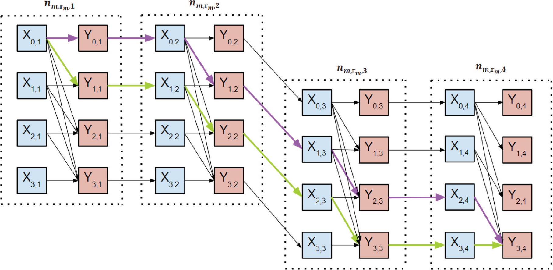
Figure 2. Example of shortest route graph
3.3. Energy Model
The energy model requires to consider the power needed for peripheral node transmission and VNF computation. When sending or receiving data between peripheral nodes, we accounted for the transmission latency alongside the electricity required. In equation (1), we represent the energy expended by communicating between two nodes as vni,vnj∈ VN, where vnij is the power expended in this communication and pdelay (linki,j ) is the transmission delay between these nodes.
In equation (2), Eidl is the energy consumed by a vn at time t when it is in its idle vstate, Emax is the energy consumed by a vn when it is in its complete state, and un (t)is the usage of a vn at time t.
Hence, the computational energy utilized in vn∈VN at t of binary variable at instance set to 1 is denoted by Bn, as given by equation (3).
Equation (4) calculates the energy usage for virtual link by the vn propagation delay pdelay (linki,j) at time t.
3.4. Cost of the Network
We represent the expense of each SFC as the total of the processing delays that all of its VNFs experience as well as the communication delays that all of its virtual connections experience. The overall cost of the system can be calculated by adding up the prices of each SFC in the system. The workload size is wvn that is used for VNF vn∈VN. If vn is determined to be vn∈Kn (s) for a particular SFC deployment selection s, then the quantity of processing capability that is allotted to v is equivalent to , and the feasibility of executing VNF vn on server m is . The latency computation in VNF vn, which is represented by Delayvn, is modeled as follows:
Under this configuration, Delayvn from equation (1) is equal to the processing delay of putting VNF vn with the workload capacity of wvn on server m with a computational ability of and is set to [0,1] of VNF vn and server m.
Delay in virtual connections; it is necessary to send data with a capacity of Dlink through each virtual connection link∈L. The latency of link in physical channel c is if and only if link∈Kn (s), in which case the bandwidth assigned to link is , as given in equation (5).
It is possible for a single virtual link to be mapped to several neighboring physical channels. The overall delay of link is determined by adding the latencies of each of the physical channels to which it is mapped. Therefore, the overall latency in virtual connection link, which we refer to as Delaylink, is calculated as follows:
The overall delay of an SFC m, which is indicated by the notation Ym (s,Ra,Rb ) is equal to the aggregate of the latencies of all of its VNFs and virtual connections in the given equation (7)
The overall fitness of the network, which is represented by the notation Y(s,Ra,Rb ), is equal to the aggregate of the latencies of each of its SFCs in the given equation (8).
Finally, equation (9) defines the objective function to reduce the latency of the network, energy consumption, and VNF data transfer from edge nodes to their outbound lines. The energy consumption calculation incorporates the processing and propagation delays, thus rendering their exclusion from the analysis.
4. The Proposed AVOAVNF
The AVOA metaheuristic method was first presented by Abdollahzadeh et al. (2021). Since that time, it has been implemented in a variety of real-world engineering applications. To build the AVOA, simulations and models were used that were based on the feeding behaviors and daily routines of African vultures. The following considerations are taken into account in order to carry out the simulation that is known as AVOA. This simulation recreates the life patterns and foraging strategies of African vultures, and it is carried out by using the following elements.
(i) There are N vultures in the African vulture population, and the user of the algorithm decides how large N should be depending on the conditions at the time of the calculation. The position space of each vulture is represented by a grid with D dimensions; the size of D varies depending on the complexity of the issue.
(ii) The population of African vultures may be broken down into three distinct clusters according to the way in which they make their livelihood. The first cluster determines the most optimal viable solution by using the fitness value of the viable solution as a metric to evaluate the quality of the approach. The second cluster of thought maintains that out of all of the potential solutions, the one that can really be implemented is the one that is second best. The third and final group is made up of the remaining vultures.
(iii) The vulture hunts in groups throughout the population in which it resides. As a direct consequence of this, several species of vultures fulfil a variety of roles within the community.
(iv) Similarly, if the fitness value of the population’s feasible solution may be understood to reflect the advantages and downsides of vultures, then the vultures who are the weakest and most hungry correspond to the vultures that are the worst at the current time. On the other hand, the vulture that is the healthiest and most numerous at this time is the greatest option. Vultures in AOVA strive to position themselves near the greatest and away from the bad.
Based on the fundamental ideas about vultures and the four assumptions used to replicate the artificial vulture’s optimization algorithm, the problem-solving process can be broken down into five stages that represent the foraging behaviours of different vultures.
4.1. Identifying the Best Vulture in Clusters
After the initial population has been formed, the fitness of each solution is determined, and the best and worst performers are chosen to serve as vultures for the first and second groups, respectively. At each iteration of the fitness test, populations are subjected to a thorough analysis.
The probability that the chosen vultures will lead the other vultures to one of the best solutions in each cluster is determined by equation (11), where P1 and P2 are the best solutions in the cluster. Both of the search operation’s input parameters must have values between 0 and 1, with the total being 1. Using the rank selection to choose the best fitness from each set using, increases the probability of selecting the optimal solution.
4.2. Vulture Hunger Rate
Vultures are remaining on the hunt for food, and when they get it, they have a burst of energy that helps them to go further in their quest for more. On the other hand, they are more aggressive when they are hungry since they lack the strength to fly long distances or to hunt for food alongside larger, stronger vultures. This sort of behavior has been modelled mathematically with the help of equation (12). The rate at which the vultures are satiated or hungry has also been used to mark the shift from the exploratory to the exploitative phase. equation (12), which accounts for the decreasing rate of satisfaction, has been used to predict this phenomenon.
In equations (12) and (13), the symbol Fv indicates that the vultures have consumed all of the food available to them, iteration i represents the number of the current iteration, itrmax represent the overall number of iterations, and m is a random value ranging from -1 to 1 that fluctuates with each new iteration. n is an integer chosen at random from the range -2 to 2. rand1 returns a result that is completely random between 0 and 1. If the z value goes below zero, it indicates that the vulture is starving, and if it goes above zero, it indicates that the vulture has satiated.
4.3. Exploration
Here, we examine the AVOA exploration phase. Vultures have keen vision, which helps them find prey and dead animals. When searching for food, vultures fly long distances and do detailed observations of their surroundings. The vultures in the AVOA may use one of two methods to explore seemingly random sites, with the method being selected at random. The exploration stage is needed to provide a value between 0 and 1 for this option before you can begin the search process. Which method is used is up to it. A random integer between 0 and 1 is created during the exploration phase and used to decide which approach to pursue. equation (14) is utilized if the number is greater than or equal to the parameter. If, however, the digit count is under equation (16), the formula will be used. This is shown by equation (17).
The position vector of a vulture in the iteration that follows will be indicated by the V(i+1), and the satiation rate of the vulture in the current iteration will be denoted by the symbol Fv, which can be determined by using equation (12). In equation (15), S(i) is a good example of the kind of vulture that is chosen by equation (17). The vultures patrol the area randomly to protect their meal from the other vultures. ε is created via the formula ε = r2, where r2 is a randomly produced number between 0 and 1, and ε is then utilized as a coefficient vector to enhance the random motion, which shifts with each iteration. r3 is a randomly generated number between 0 and 1. The vector location is determined by the vulture’s V1. The variable boundaries are shown by LB and UB. r3 increases the amount of unpredictability. If r3 is somewhat close to 1, solutions that are comparable are spread, which adds a random motion to the LB.
4.4. Exploitation Stage-1
At this point, the AVOA’s efficiency stage is being analyzed for its effectiveness. The AVOA will proceed to the exploitation phase if the value of Fv is less than 1, since this indicates that there is room for profit. This phase, like the previous one, is divided into two sections, and each of those portions employs a distinct tactic. Two factors, V2 and V3, define the likelihood that each approach will be selected throughout each of the phases that take place internally. The strategy for the first phase is determined by the parameter V2, whereas the second phase is determined by the parameter V3. Both of the parameters need to be set to 0 and 1 before the search operation can be carried out. When the value of |Fv| is between 1 and 0.5, the exploitation phase starts. During the initial phase of the battle, both a rotating flying strategy and a siege-fighting strategy will be used. Before performing a searching operation, the value of V2, which ranges between 0 and 1, will be used to choose which strategy to use. rv2 is constructed right at the beginning of this phase. If this amount is more than or equal to V2, the implementation of the Siege-fight will go more slowly. In the event that the random number is lower than V2, the rotating flying method will be used. Equations (18) and (19) illustrate how to carry out this technique.
The value of D(i) may be found by using equation (15), and the value of Fv can be found by applying equation (12) to the satiation rate of vultures. A random number between 0 and 1, r4 is added to the formula to make the random coefficient even more unpredictable. In equation (18), S(i) represents one of the best vultures from the two groups that was chosen using equation (19) during the current iteration. V(i) represents the current vector location of the vulture, which is used to calculate the distance between the vulture and one of the best vultures from the two groups.
Vultures typically perform a flying pattern that may be described as a rotating flight, and this flight pattern can be utilized to mimic spiral motion. Mathematical modelling of circular flight has been accomplished via the use of the spiral model. Using this approach will result in the formation of a spiral equation (23) involving all of the vultures and one of the top two vultures. Equations (20) and (21) are used to compute a1 and a2 and provide an expression for the rotational flight.
4.5. Exploitation Stage-2
During the second stage of the exploitation process, the movements of the two vultures lure many other species of vultures to the food supply, where a siege and a vigorous fight for food ensue. When the value of Fv is lower than 0.5, the transition into this phase begins. During this step, the random number generator rv3 will produce a value between 0 and 1. If rv3 is more than or equal to V3, a large number of different kinds of vultures should converge around the source of food. Alternately, the aggressive siege-fight approach described in equation (28) is adopted if the value created is less than V3. This occurs if the value generated is less than V3.
In the last step, the vultures are summed up with the help of equation (25), in which A1 and A2 come from the previous equations (24) and (25), and V(i+1)is the vulture vector for the next iteration. The names given to the best vultures in the first and second groups of this iteration are Bestv1 (i) and Bestv2 (i), respectively. V(i) stands for the vector position of a vulture at any given moment.
When the value of |Fv| is more than 0.5, the head vultures begin to hunger, and as a result, they are unable to compete with the other vultures in terms of strength. Equation (27) is utilized to simulate this motion as accurately as possible. d(t) represents the distance that the vulture is from one of the best vultures in the two groups, and this distance is determined by applying equation (26) to the equation found in equation (27). Patterns of Levy flight [40] have been exploited to improve the performance of the AVOA in Eq. (28), and LF has been recognized and used in the operations of metaheuristic algorithms.
The fitness of a solution to a vulture may be determined by assessing the fitness function , which is considered in the following equation (29).
4.6. Pseudocode of the AVOAVNF
The pseudocode for the proposed AVOAVNF algorithm is shown in Algorithm 1. The proposed algorithm takes and returns the highlighted phrases as input and output.
Input: Physical network G = (Sp,∁n ), SFC topology G=(VNm,linkm ), each vulture v∈Vn
Output: Bestv
1. Begin
2. Initialization of population size Vn.
3. for each vulture v∈Vndo /*Loop to check termination */
4. Calculate /*Using equation (29) */
5. end for
6. Set t=1, itrmax
7. for t≤itrmax do
8. for each vulture v∈Vn do
9. if (|Fv| ≥ 1) then
10. if (V1 ≥ r_(v1)) then
11. Update position V(i) using Equation (14)
12. else
13. Update position V(i) using Equation (16)
14. if (|Fv| < 1) then
15. if (|Fv| ≥ 0.5) then
16. if (V2≥ r_(v2)) then
17. Update position V(i) using Equation (18)
18. else
19. Update position V(i) using Equation (22)
20. else
21. if (V3 ≥ rv3 ) then
22. Update position V(i) using Equation (26)
23. else
24. Update position V(i) using Equation (27).
25. end for
26. t=t+1
27. end for
28. for i= 1: Vn do
29. For i= 1: Nω do
30. If F(i+1) < F(i) then
31. Bestv= F(i+1)
32. Else
33. Bestv= V(i)
34. end for
35. end for
36. end for
37. end
Algorithm 1 represent the Input: Physical network G=(S_p,∁_n), SFC topology G=(〖VN〗_m,〖link〗_m), each vulture v ∈V_n Output: 〖Best〗_v(finding the shortest route) and begins by initializing the population size N_ω in its first line. From lines 3-7 to establish the position vector for each vulture v ∈V_n, taking into account all constraints. Subsequently, the optimal value of position vectors for the vultures is selected according to their respective fitness values, utilizing the sorting algorithm as selected. The position V(i) of each vulture in the dimension was updated in every iteration, as indicated by lines 8-10. Update vultures’ position V(i) using equations 14 and 16, 18 and 22, and equation 26-27 in its line 11-24. Subsequently, the parameters’ values are revised in line 17, followed by the computation of the fitness value. Subsequently, the three optimal solutions are updated. After every iteration, and position of the vulture, are updated, it means that a new population of vultures is created and again their best fitness is calculated and accordingly the best fitness is updated (line 27-33). Upon completion of all iterations, the optimal placement of each SFC within the edge network is determined. Finally, the solution vector 〖Best〗_v is transformed.
5. Simulation Setup and Result Analysis
The performance of the proposed AVOA-based architecture for SFC placement is given, studied, and assessed in extensive detail in this section. To evaluate the quality of the answers that the proposed algorithm generates, a comprehensive and diversified collection of tests has been carried out. These experiments have been carried out under a variety of network topologies and algorithm settings. It is important to point out that the experiment configurations were chosen so as to imitate a wide variety of real-world settings, such as Industry 4.0, in terms of the network architecture, the number of physical hosts, as well as the demand for resources and the availability of those resources. The MATLAB simulation program was used to design the AVOA framework that has been proposed. The tests were run on a computer with an Intel(R) Core i5 central processing unit operating at 2.8 GHz and 8 gigabytes of random-access memory. In the first phase of this process, we have analyzed the proposed framework and made any necessary adjustments in terms of the population size of the AVOA algorithm that has been chosen for the AVOA configuration. All of AVOAVNF setup settings are shown in Table 1. In this section, the proposed algorithm is tested using a variety of different numbers of nodes, including 50, 100, and 150, and is compared against several benchmark approaches. The amount of SFC requests that are allowed might be impacted by the number of nodes. In particular, a large number of nodes in the edge network denotes ample resources, and it often results in a reduction in the number of unsuccessful SFCs. However, certain requests may not be deployed in simulations with a limited number of nodes. It is anticipated that the proposed method would be more compatible with SFC requests when the number of nodes is minimal. This is because VNF is reused throughout the process. It is typical practice to investigate simulations using varying numbers of nodes.
Table 1. Simulation parameters
Parameters |
Values |
Number of edge nodes |
200 |
Memory resource |
1 GB |
CPU resource |
1000 |
Bandwidth per each node |
1800 mbps |
Number of SFC type |
10 |
Number of VNF type |
1-8 |
Number of SFC requested |
1000 |
VNF in an SFC |
1-8 |
Packet size |
4000 kbps |
Delay threshold request |
100 ms |
VNF & SFC time out |
2 min |
Simulation runs |
30 |
w |
2.5 |
Population size |
30 |
Initial position of the vulture |
0.5 |
5.1. Performance Result Evaluation
In this part, we will evaluate the outcomes of the AVOAVNF algorithm based on how they compare to state-of-the-art techniques such as BGWO (Shahjalal et al., 2022), DDRL, BIP (Akhtar et al., 2021) and MILP (Magoula et al., 2021). The evaluation is carried out using a number of performance indicators, including energy consumption, throughput, resource cost, execution time, and end-to-end delay cost. A series of comparisons to validate the efficacy of the proposed approach are shown in Fig.3 to Fig.8, respectively. The presented data encompasses various comparisons, including those based on reward, energy consumption, throughput, delay cost, resource cost, and execution time. The performance indicators for each comparison are presented based on the aggregate number of requests. Furthermore, the comparisons are repeated based on three discrete scenarios that encompass the overall count of unique nodes, specifically 50, 100, and 150.
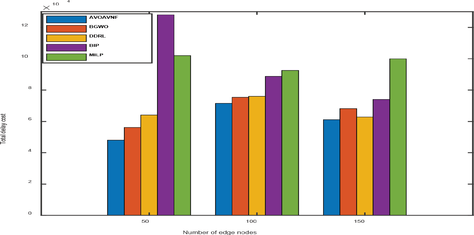
Figure 3. Performance analysis of delay cost
The proposed technique achieves superior results when the number of nodes is kept to a minimum, and it significantly lowers both the cost of delay and the number of resources required while preserving throughput. In point of fact, the proposed algorithm with efficient placement has been successful in successfully distributing resources in an appropriate manner in the face of resource shortage. It has been determined that the AVOAVNF algorithm has an energy consumption rate that is superior to BGWO, DDRL, BIP, and MILP by a margin of 8.35%, 12.23%, 29.54%, and 52.29%, respectively. In comparison to the benchmark approaches, the energy efficiency of SFCs has been enhanced thanks to the algorithm that was provided. This has resulted in an improvement in the supply of services. Increasing the number of nodes, on the other hand, is said to result in a much cheaper resource cost by the technique that was presented. As a result, the proposed technique, when implemented in fog networks with enough resources, is able to allocate VNFs to the nodes that are the most appropriate for them. When compared to the benchmark approaches in terms of the resource cost, the proposed algorithm performs much better overall. This improvement ranges from 15% to 30%.
As can be seen, the MILP technique has the lowest performance across the board when compared to other approaches. The wasteful use of resources caused by a strategy to recycling VNFs that is motivated only by greed is the root cause of this problem. In addition, the deployment of VNFs over MILP requires additional nodes, which drives up the cost of delay. It is reasonable to anticipate that RF will have a poor throughput given the significant number of resources it requires. Although BGWO and DDRL produces superior outcomes than MILP, this approach initializes a greater number of nodes since it chooses the shortest pathways. According to the findings, the resource costs incurred by the BGWO and DDRL due to the large number of nodes have significantly grown, which has resulted in a decrease in the pay-out. The performance of the BIP approach is comparable to that of the BGWO and DDRL in the majority of simulations; nevertheless, its performance is inferior to that of the proposed algorithm since it is not as effective due to its lack of consideration for SFC deployment.

Figure 4. Performance analysis of throughput
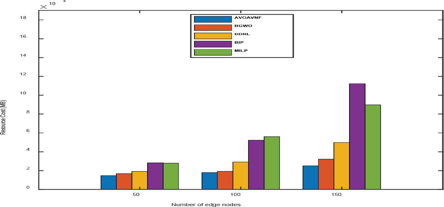
Figure 5. Performance analysis of resource cost
During this experiment, our goals were to assess the total energy used by each placement algorithm and determine whether or not our strategy was able to provide placement plans that are energy efficient. Fig. 6 demonstrates that our method uses less energy than the other methods, despite the fact that it fulfils a greater number of requests that have been filed. The VNF sharing mechanism contributes to the achievement of this outcome since it requires a smaller number of edge nodes to fulfil a predetermined number of requests, while greedy and random often choose VNF instances that are dispersed among a greater number of edge nodes. When there are more than 1000 requests, the environment’s resources become depleted, and all placement options use the same amount of energy. This is the behavior that is anticipated for the extreme situation that has been provided.
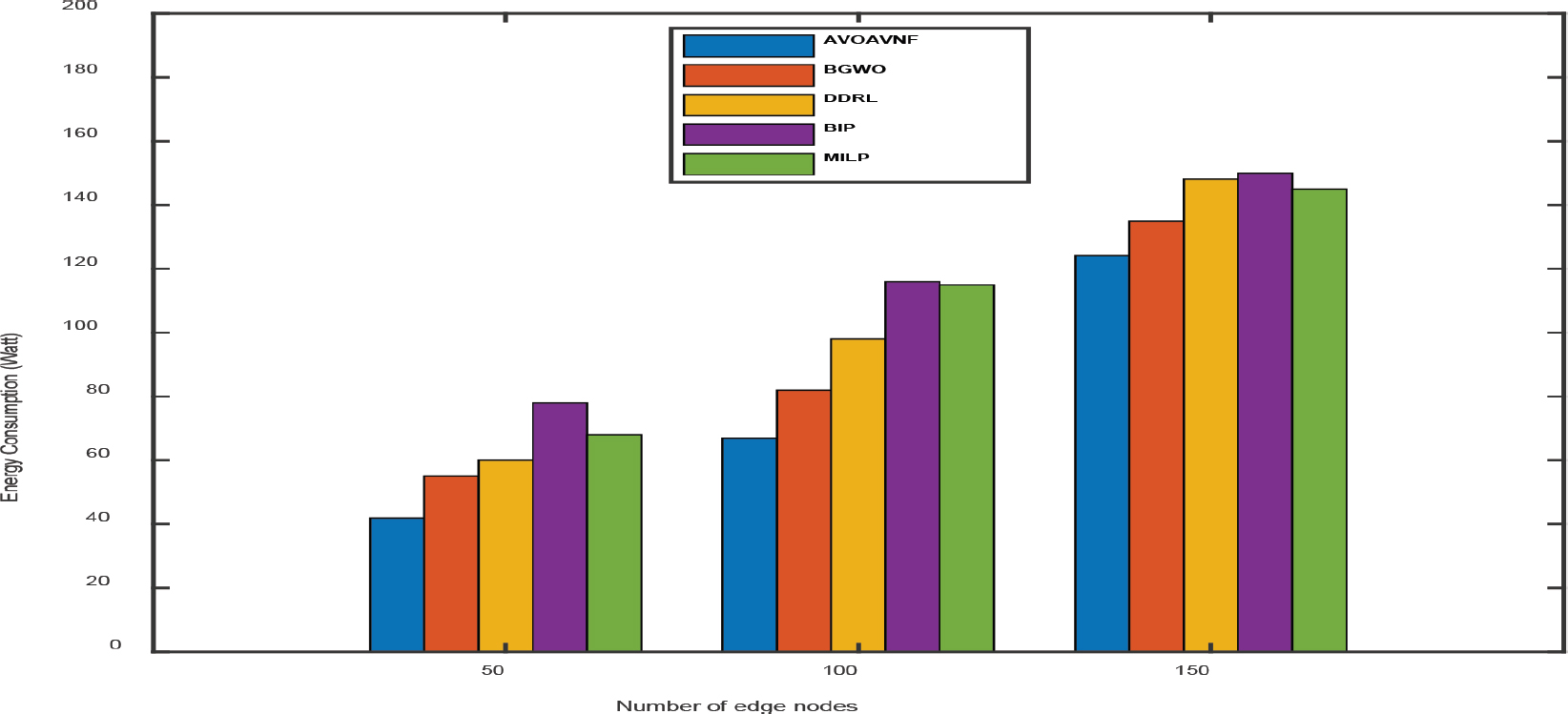
Figure 6. Energy consumption analysis of AVOAVNF vs. existing methods
The proposed algorithm’s execution time was variable and was based on the degree of difficulty of the edge network as well as the configuration of the SFC. The time needed by the proposed technique to process 1000 SFC requests was around 52 seconds when using a modest number of nodes. In spite of this, the proposed method did not experience a discernible lengthening of its execution time with an increase in the number of nodes. The use of VNFs may provide an explanation for this phenomenon, particularly when one takes into account the dynamic distribution of VNFs and the allocation of nodes based on it. Although BGWO, DDRL, BIP, and MILP have lower runtimes than the proposed method because they employ the shortest route when placing nodes in networks with a low number of nodes, placing nodes in networks with a big number of nodes needs a significant amount of runtime. In addition, runtime for MILP is quite low since it employs a greedy strategy and is able to process requests in a short amount of time. Despite the fact that MILP has a shorter runtime than the approach that was presented, its performance is much worse.
The BIP algorithm had the slowest runtime of the ones that were compared. BIP has a relatively long runtime because it requires a substantial amount of data processing to be performed on each request before it can interact with significant networks. As can be seen in the illustration, the amount of time required to complete this procedure has grown exponentially along with the number of nodes.

Figure 7. Execution time analysis of AVOAVNF vs. existing methods
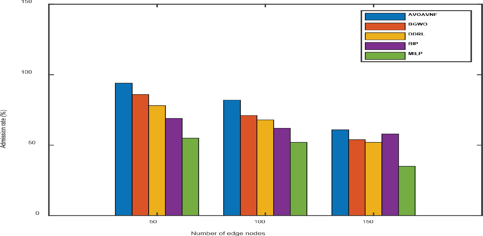
Figure 8. Performance analysis of SFC admission rate
6. Conclusion
In this paper, the AVOA methodology for the deployment of SFC within the framework of the cloud-edge computing architecture. The present study aims to achieve equilibrium between the deployment cost of virtual network functions (VNFs) for users and the limitations imposed by an edge computing environment, while also accounting for user mobility across edges. The objective is to devise a placement strategy for service chains that mitigates energy consumption, enhances throughput, minimizes resource cost, reduces execution time, and adheres to end-to-end delay constraints. This study presents a comprehensive formulation of the optimization problem and proposes a solution to the SFC placement problem through the utilization of the AVOA algorithm. The proposed method is designed to address the issue of complexity and is further enhanced with an early stopping criterion, position awareness, and solution filtering. The AVOAVNF methodology enhances performance by optimizing computer resources relative to conventional techniques, as evidenced by comprehensive simulations conducted on edge networks.
To accomplish its goals, the algorithm considers latency, computing resource capacity, and energy usage. Thus, possible edge nodes are assessed for VNF hosting based on their properties. The method outperforms BGWO, DDRL, BIP, and MILP and provides more customizable solutions. The AVOAVNF method outperforms the existing techniques by 8.35%, 12.23%, 29.54%, and 52.29%. Edge computing requires QoS due to edge nodes’ power constraints and energy usage. Our future work comprises three crucial elements. First, we want to apply our model to handle ongoing user SFC requests. Second, we want to detect user motion and respond accordingly. Finally, we will provide a technique to dynamically alter the number of SFCs that may share a VNF instance depending on workload.
Conflict of interest
All authors have no conflict of interest to report.
References
Abbas, N., Zhang, Y., Taherkordi, A., & Skeie, T. (2017). Mobile Edge Computing: A survey. IEEE Internet of Things Journal, 5(1), 450–465. https://doi.org/10.1109/JIOT.2017.2750180
Abdollahzadeh, B., Gharehchopogh, F.S., & Mirjalili, S. (2021). African vulture’s optimization algorithm: A new nature-inspired metaheuristic algorithm for global optimization problems. Computers & Industrial Engineering, 158, 107408. https://doi.org/10.1016/j.cie.2021.107408
Akhtar, N., Matta, I., Raza, A., Goratti, L., Braun, T., & Esposito, F. (2021). Managing chains of application functions over Multi-Technology edge networks. IEEE Transactions on Network and Service Management, 18(1), 511–525. https://doi.org/10.1109/TNSM.2021.3050009
Ale, L., Zhang, N., Fang, X., Chen, X., Wu, S., & Li, L. (2021). Delay-Aware and Energy-Efficient computation offloading in Mobile-Edge Computing using deep Reinforcement learning. IEEE Transactions on Cognitive Communications and Networking, 7(3), 881–892. https://doi.org/10.1109/TCCN.2021.3066619
Almurshed, O., Rana, O., & Chard, K. (2022). Greedy Nominator Heuristic: Virtual function placement on fog resources. Concurrency and Computation: Practice and Experience, 34(6), e6765. https://doi.org/10.1002/cpe.6765
Attaoui, W., Sabir, E., Elbiaze, H. and Guizani, M., 2022. VNF and Container Placement: Recent Advances and Future Trends. arXiv preprint arXiv:2204.00178.
Bahreini, T., & Grosu, D. (2020). Efficient Algorithms for Multi-Component application placement in mobile edge Computing. IEEE Transactions on Cloud Computing, 10(4), 2550–2563. https://doi.org/10.1109/tcc.2020.3038626
Cziva, R., & Pezaros, D. P. (2017). Container network functions: Bringing NFV to the network edge. IEEE Communications Magazine, 55(6), 24–31. https://doi.org/10.1109/MCOM.2017.1601039
Deng, S., Xiang, Z., Taheri, J., Khoshkholghi, M. A., Yin, J., Zomaya, A. Y., & Dustdar, S. (2021). Optimal application deployment in resource constrained distributed edges. IEEE Transactions on Mobile Computing, 20(5), 1907–1923. https://doi.org/10.1109/tmc.2020.2970698
Gao, X., Liu, R., & Kaushik, A. (2022). Virtual network function placement in satellite edge computing with a potential game approach. IEEE Transactions on Network and Service Management, 19(2), 1243–1259. https://doi.org/10.1109/TNSM.2022.3141165
Hazra, A., Adhikari, M., Amgoth, T., & Srirama, S. N. (2021). Intelligent Service Deployment Policy for Next-Generation Industrial Edge Networks. IEEE Transactions on Network Science and Engineering, 9(5), 3057–3066. https://doi.org/10.1109/tnse.2021.3122178
Khan, W. Z., Ahmed, E., Hakak, S., Yaqoob, I., & Ahmed, A. (2019). Edge Computing: a survey. Future Generation Computer Systems, 97, 219–235. https://doi.org/10.1016/j.future.2019.02.050
Khoshkholghi, M. A., Khan, M. G., Noghani, K. A., Taheri, J., Bhamare, D., Kassler, A., Xiang, Z., Deng, S., & Yang, X. (2020). Service function chain placement for joint cost and latency optimization. Mobile Networks and Applications, 25(6), 2191–2205. https://doi.org/10.1007/s11036-020-01661-w
Khoshkholghi, M. A., & Mahmoodi, T. (2022). Edge Intelligence for service function chain deployment in NFV-enabled networks. Computer Networks, 219, 109451. https://doi.org/10.1016/j.comnet.2022.109451
Kouah, R., Alleg, A., Laraba, A., & Ahmed, T. (2018). Energy-aware placement for iot-service function chain. 2018 IEEE 23rd International Workshop on Computer Aided Modeling and Design of Communication Links and Networks (CAMAD), 1–7. IEEE. https://doi.org/10.1109/CAMAD.2018.8515003
Liang, W., Cui, L., & Tso, F. P. (2022). Low-latency service function chain migration in edge-core networks based on open Jackson networks. Journal of Systems Architecture, 124, 102405. https://doi.org/10.1016/j.sysarc.2022.102405
Luizelli, M. C., Cordeiro, W., Buriol, L. S., & Gaspary, L. P. (2017). A fix-and-optimize approach for efficient and large scale virtual network function placement and chaining. Computer Communications, 102, 67–77. https://doi.org/10.1016/j.comcom.2016.11.002
Magoula, L., Barmpounakis, S., Stavrakakis, I., & Alonistioti, N., (2021). A genetic algorithm approach for service function chain placement in 5G and beyond, virtualized edge networks. Computer Networks, 195, 108157. https://doi.org/10.1016/j.comnet.2021.108157
Matias, J., Garay, J., Toledo, N., Unzilla, J., & Jacob, E. (2015). Toward an SDN-enabled NFV architecture. IEEE Communications Magazine, 53(4), 187–193. https://doi.org/10.1109/MCOM.2015.7081093
Munusamy, A., Adhikari, M., Balasubramanian, V., Khan, M. A., Menon, V. G., Rawat, D., & Srirama, S. N. (2021). Service deployment strategy for predictive analysis of FinTech IoT applications in edge networks. IEEE Internet of Things Journal.
Pei, J., Hong, P., Pan, M., Liu, J., & Zhou, J. (2019). Optimal VNF placement via deep reinforcement learning in SDN/NFV-Enabled networks. IEEE Journal on Selected Areas in Communications, 38(2), 263–278. https://doi.org/10.1109/jsac.2019.2959181
Pham, C., Tran, N. H., Ren, S., Saad, W., & Hong, C. S. (2017). Traffic-Aware and Energy-Efficient VNF placement for service chaining: joint sampling and matching approach. IEEE Transactions on Services Computing, 13(1), 172–185. https://doi.org/10.1109/tsc.2017.2671867
Qu, H., Wang, K., & Zhao, J. (2022). Priority-awareness VNF migration method based on deep Reinforcement learning. Computer Networks, 208, 108866. https://doi.org/10.1016/j.comnet.2022.108866
Sahoo, B. M., Pandey, H. M., & Amgoth, T. (2022). A genetic algorithm inspired optimized cluster head selection method in wireless sensor networks. Swarm and Evolutionary Computation, 75, 101151. https://doi.org/10.1016/j.swevo.2022.101151
Schardong, F., Nunes, I., & Schaeffer-Filho, A. (2021). NFV Resource Allocation: A Systematic Review and Taxonomy of VNF forwarding graph embedding. Computer Networks, 185, 107726. https://doi.org/10.1016/j.comnet.2020.107726
Shahjalal, M., Farhana, N., Roy, P., Razzaque, M. A., Kaur, K., & Hassan, M. M. (2022). A binary Gray Wolf optimization algorithm for deployment of virtual network functions in 5G hybrid cloud. Computer Communications, 193, 63–74. https://doi.org/10.1016/j.comcom.2022.06.041
Tajiki, M. M., Salsano, S., Chiaraviglio, L., Shojafar, M., & Akbari, B. (2018). Joint Energy Efficient and QOS-Aware path allocation and VNF placement for service function chaining. IEEE Transactions on Network and Service Management, 16(1), 374–388. https://doi.org/10.1109/TNSM.2018.2873225
Tomassilli, A., Giroire, F., Huin, N., & Pérennes, S. (2018). Probably efficient algorithms for placement of service function chains with ordering constraints. IEEE INFOCOM 2018 – IEEE Conference on Computer Communications, 774–782. IEEE. https://doi.org/10.1109/INFOCOM.2018.8486275
Wang, M., Cheng, B., Feng, W., & Chen, J. (2019). An efficient service function chain placement algorithm in a MEC-NFV environment. 2019 IEEE Global Communications Conference (GLOBECOM), 1–6. IEEE. https://doi.org/10.1109/GLOBECOM38437.2019.9013235
Wang, S., Zafer, M., & Leung, K. K. (2017). Online placement of Multi-Component applications in edge computing environments. IEEE Access, 5, 2514–2533. https://doi.org/10.1109/access.2017.2665971
Wang, X., Ning, Z., Guo, L., Guo, S., Gao, X., & Wang, G. (2021). Online learning for distributed computation offloading in wireless powered mobile edge computing networks. IEEE Transactions on Parallel and Distributed Systems, 33(8), 1841–1855. https://doi.org/10.1109/tpds.2021.3129618
Yang, B., Chai, W. K., Pavlou, G., & Katsaros, K.V. (2016, October). Seamless support of low latency mobile applications with nfv-enabled mobile edge-cloud. 2016 5th IEEE International Conference on Cloud Networking (Cloudnet), 136–141. IEEE. https://doi.org/10.1109/CloudNet.2016.21
Yang, S., Li, F., Trajanovski, S., Chen, X., Wang, Y., & Fu, X. (2019). Delay-aware virtual network function placement and routing in edge clouds. IEEE Transactions on Mobile Computing, 20(2), 445–459. https://doi.org/10.1109/TMC.2019.2942306
Yang, X. S. (2010). Firefly algorithm, Levy flights and global optimization. In Research and development in intelligent systems XXVI: Incorporating applications and innovations in intelligent systems XVII (pp. 209–218). Springer London. https://doi.org/10.1007/978-1-84882-983-1_15
Zahedi, S. R., Jamali, S., & Bayat, P. (2022). EMCFIS: Evolutionary Multi-criteria Fuzzy Inference System for virtual network function placement and routing. Applied Soft Computing, 117, 108427. https://doi.org/10.1016/j.asoc.2022.108427
Zhang, S., Jia, W., Tang, Z., Lou, J., & Zhao, W. (2022). Efficient instance reuse approach for service function chain placement in mobile edge computing. Computer Networks, 211, 109010. https://doi.org/10.1016/j.comnet.2022.109010
Zhang, Y., Zhang, F., Si, T., & Rezaeipanah, A. (2022). A dynamic planning model for deploying service functions chain in Fog-cloud computing. Journal of King Saud University - Computer and Information Sciences, 34(10), 7948–7960. https://doi.org/10.1016/j.jksuci.2022.07.012