ADCAIJ: Advances in Distributed Computing and Artificial Intelligence Journal
Regular Issue, Vol. 12 N. 1 (2023), e31206
eISSN: 2255-2863
DOI: https://doi.org/10.14201/adcaij.31206

Ensemble Learning Approach for Effective Software Development Effort Estimation with Future Ranking

K. Eswara Rao^a, Balamurali Pydi^b, P. Annan Naidu^c, U. D. Prasann^d, P. Anjaneyulu^e

^{a b c e}Dept.of CSE, Aditya Institute of Technology and Management, Srikakulam, AP, India, 532201.
^dDept.of EEE, Aditya Institute of Technology and Management, Srikakulam, AP, India, 532201.
eswarkoppala@gmail.com, balu_p4@yahoo.com, annanpaidi@gmail.com, udprasanna@gmail.com, annanpaidi@gmail.com

ABSTRACT

KEYWORDS

1. Introduction

Software development is crucial to critical areas of global management due to the SDEE’s rising need for high-quality products and software programmes. A few systems employ software metrics as part of their SDEE with the unique purpose of creating acceptable software that prioritizes efficiency in dynamic settings (Azath, H. et al., 2018), (Pospieszny P. et al., 2018). The challenge is evaluating those metrics early in the project lifecycle when the limits of each effort must be determined, and there are significant uncertainties about the end product’s functionality. Actions taken in these scenarios may have unrealistic views, such as “underestimating” a plan of action, which could lead to delays, going over budget, delivering a defective product, and so on (Mustapha, H., 2019). Effort estimation techniques include user-point story (M.A. Kuhail et al., 2022), COCOMO (S. Denard et al., 2020), functional point (V.V. Hai et al. 2021), Line of Code (L. Mak et al., 2022), and others. COCOMO is the most popular standard SEE among the software engineering community (C. Rosen et al., 2020). Another difficulty is working with the team and predicting their vitals, which is tricky and stochastic. Another is identifying potential risks (Abdulmajeed, A. A. et al., 2021) and (El Bajta, M., & Idri, A., 2020). The accuracy of this method depends on how closely the new initiative aligns with the expert’s field of expertise. Ensemble and soft computing approaches can address the issues encountered when employing algorithmic and expert judgement methods and are constantly on the rise to solve all critical problems (A. Mashkoor et al., 2022). However, ensemble use is too difficult due to issues related to the dependability of the achieved predictive accuracy score.

Furthermore, various ensemble techniques have beneficial and limiting characteristics, yet their adoption is still in its early stages. As a result, the proposed scheme introduces a novel learning-based SDEE method aimed at overcoming estimation weak points in existing schemes and addressing computational efficiency when deploying learning schemes. Therefore, the proposed scheme introduces a novel SDEE method meant to overcome the estimation loopholes in existing schemes and address the computational efficiency while deploying learning schemes. The following are the proposed scheme’s novelty and contribution: The research model constructs a predictive model using advanced machine learning-based feature optimization discretely towards developing a framework. The proposed scheme introduces an SDEE computational framework that enables an estimator to perform simplified predictive effort estimation for their target software product.

The following sections, including two significant discoveries, comprise the rest of this study. Section 2 discusses the literature-related research on estimation techniques for software development effort estimation that has been done. The ML models (LR, k-NN, MLP, RF, DT, NB, and SVM) that were considered to combine some of the best features of the suggested method are examined in Section 3, and a stacked ensemble learning model for SDEE is built in Section 4. It summarizes the results of the studies and demonstrates the experimental setup in Section 5. The research is concluded in Section 6, along with its future scope.

2. Literature Report

This section describes summary of ML strategies is offered after a study of general effort estimation algorithms concludes with a review of various classification methods and methodologies, as well as a comparison of ways that can be used to estimate software development effort.

2.1. ML for SDEE

Investigated several data sets and obtained encouraging findings for software development effort assessment. When estimating software maintenance effort using particle swarm optimization, (Singh, C., et al., 2019) proposed a successful swarm intelligence-based method. Undefined constraints, product quality, massive organizational involvement, overestimation, and underestimation are some of the major problems with current methods, despite the fact that the standard techniques of SDEE are readily available, as explained in the preceding section. It should be noted that the issues raised above could be related to the majority of the current standard SDEE techniques even though there isn’t a fully effective way to control them yet. The research that has already been done to advance SDEE techniques is discussed in the section that follows, along with its advantages and disadvantages.

2.2. Evolutionary strategy

Many recent studies have emphasized considering the linkage between allocating human resources and SEE to decide on outsourcing the projects for faster delivery. The solution to this problem is seen in the work of (H. Y. Chianget et al., 2020) where an integer-based programming methodology has been used for formulating a decision process. For prediction, networks (RBFNN) were utilised. This project produced a conclusion that the UCP method’s environmental considerations are ideal for software system productivity forecasting. Existing SEE schemes are often said to adopt learning-based techniques to estimate effort. (H. D. P. De Carvalho, et al., 2021) have used an extreme learning machine to identify all the essential parameters that potentially influence the SCE technique. The study utilized various machine learning approaches to improve effort estimation. These approaches outperformed Multi-Layer Perceptron, Logistic Regression, Support Vector Machine, and K-Nearest Neighbouring in terms of estimation accuracy. Machine learning is implemented in Software Component Engineering to reduce testing time and identify fewer bugs.

The authors suggest using analogy-based techniques for estimating accuracy and environment in software development. They found that when paired with fuzzy logic, a strategy called ASEE produced the desired results. Another strategy called 2FA-K proto-types was proposed by different authors, and its outcomes were evaluated using four datasets. The study found that the 2FA-K prototypes and modes were more effective than traditional analogy techniques for generating the necessary output. The authors introduced a new method for estimating effort based on multiple datasets, with a focus on minimizing failure and cost. They used the Artificial Bee Colony technique to select neural network weights and evaluated the algorithm’s performance using Mean Absolute Relative Error and Mean Magnitude of Relative Error.Fuzzy logic and input variables are used in the methodology based on analogy suggested in (Idri, A., et al., 2002) to manage both numerical and fuzzy data. Utilizing categorical variables from COCOMO 81 data, the methodology is validated. In essence, estimation by analogy is a type of case-based reasoning (CBR). The foundation of CBR is based on the concept that similar software projects require similar amounts of work. In a fuzzy analogy, fuzzy variables are used. This process involves three steps: identifying a case, determining the best feature weighting using ABE, and evaluating accuracy using PRED and MMRE metrics. It is important for a cost estimation approach to be accepted and trusted by practitioners and produce accurate estimates in order for it to be beneficial. The suggested methods increase accuracy and reliability and eliminate unnecessary features. The study used various sets of real-world data.

Other Techniques

There are various methods for estimating software development effort, in addition to those mentioned in Table 1. These methods use different software datasets to estimate the work required for a software project and also use various approaches and metrics to improve performance.

3. Research Methodology

The proposed approach is followed by two phases: first is, objective of proposed work by using Random Forest and Gradient Boost based algorithms for remove weakest features with take support of feature-ranking method, and in the second-phase, proposed an advanced stacked ensemble model for software development effort estimation. Figure 1 shows the overall process of feature selection and software development effort estimation.

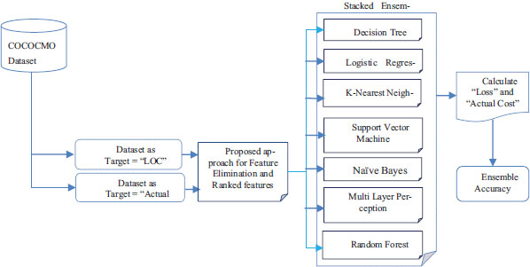
3.1. Proposed Model

This research aims to demonstrate the benefits of selecting specific features based on their ranking, and to present a majority of features that can accurately predict these ranked features when using improved learning algorithms. The model with fewer features helps to avoid unnecessary ones, without using a specific standard to exclude features. The user can specify the number of predictor subsets to determine the subgroup size and compute the performance. The model is then trained using the best subset, eliminating any dependencies and co linearity. Tree learning techniques are proposed to address the challenge of optimal feature selection, particularly for imbalanced data in a software-quality dataset. The research defines several feature selection phases to achieve these objectives.

3.2. Feature Selection

An effective system for finding the features that will be used in the training of the models is the feature selection approach (Has an, M. A. M., et al., 2016). The approach used in the COCOMO-81 dataset involves selecting the most important features for the model by ranking them based on their importance. This process is repeated until the model has the necessary number of features. The approach splits the features into two sets and examines fifteen features with different targets. The goal is to avoid using the weakest features and reduce the number of features used in the model. There are no specific criteria for dropping features, but the precision of the approach improves as more predictor subsets are utilized. The proposed approach utilizes random forest and gradient tree boost methods to select features that are common or similar to each other and create a new optimized dataset for the ensemble model in the second phase.. To support the first phase, the following Algorithm 1 and Algorithm 2 are taken.

Algorithm 1. Pseudo Code of Random Forest Feature Selection

 Input:

        Dataset D={(x₁, y₁), (x₂, y₂),…,(x_n, y_n),} where x_i ∈ R^p and y_i ∈ {-1,+1}

        Set of α features F_e= {x₁,x₂,…,x_α}

 Output:

        To assign rankings of features R = (D, {r_x1, r_x2…r_xα})

 Begin :

1: Draw N_tree bootstrap samples from the training of n samples.

2: modified each bootstrap with random sample m_try Measure the feature importance

3: for i ← 1 to x_e do

4: each tree t of the k^th RF consider the associated OOB_t sample

5: Compute Err_OOBt) error of single tree t on this OOB_t sample

6: Randomly permute $x_j=OO{B}_t^j$

7: Compute Err_OOBt of x_j

8: Calculate $PI{M}_k\left(x_j\right)=\frac{1}{n_{tree}}\sum _t(Er{r}_{OO{B}_t^j}-Er{r}_{OO{B}_t})$

9: Find $APIM\left(x_j\right)=\frac{1}{n_{tree}}\sum _{k=1}^{n}PI{M}_k\left(x_j\right)$

10: return R = {r_x1,r_x2 …r_xn} based on APIM(x_j )

11: end for

       The resulting model outputs are used as the final forecast for test cases.

       Note: Ranking assigned from 1 to 10.

End

Algorithm 2: Pseudo Code of Gradient Boost Feature Selection

 Input:

        Dataset D={(x₁,y₁),(x₂,y₂),…,(x_n,y_n),} learning rate ∈ iterations ⊺

        Set of α features F_e= {x₁,x₂,…,x_α}

 Output:

        To assign rankings of features R = (D, {r_x1, r_x2…r_xα})

 Begin :

1: Let Η be the set of all possible regression trees.

2: Inputs are mapped to ϑ^H through ϕ(X)=[h₁(X),…..,h_|H|(X)]^⊺

3: for t=1 to ⊺ do

4: calculate $\underset{\beta }{min}\sum _{\left(\varphi \right(x_i),y_i)},l\left(\varphi \right(x_i),y_{i,\beta })+\lambda |\beta {|}_1+\mu q_{\in }(\beta )$

                                                                where β is a sparse linear vector

5: computer Final classifier $H\left(x\right)=\sum _{t=0}^t{\beta }_{\tau }{h}_{\tau }\left(x\right)$ For first ⊺ entries β != 0

6: Extracted feature $F_e=\sum _{t=1}^T\left|F_{ft}{\beta }_t\right|$

7: modified q_∈(β) and update H = H + ∈h_⊺

8: for each feature f used in h_τ, set θ_f= 0 and Ω = Ω ∪ f

9: calculate optimization $\underset{\beta }{min}\sum _{\left(\mathrm{\varphi }\right(X_i),{\mathrm{y}}_{\mathrm{i}}),}l(\varphi \left(x_i\right),y_i,\beta )+\lambda |\beta {|}_1+\mu q_{ϵ}(\beta )$

10: end for

11: return R = {r_x1, r_x2 …r_xn}

                            based on ${\mathrm{h}}_{\mathrm{T}}=\underset{{\mathrm{h}}_{\mathrm{T}}\mathrm{T}\mathrm{H}}{\mathrm{argmin}}\frac{1}{2}\sum _{\mathrm{i}=1}^{\mathrm{n}}{({\mathrm{g}}_{\mathrm{i}}-{\mathrm{h}}_{\mathrm{T}}\left({\mathrm{x}}_{\mathrm{i}}\right))}^2+\mathrm{\mu }\sum _{\mathrm{f}=1}^{\mathrm{d}}{\mathrm{\varphi }}_{\mathrm{f}}{\mathrm{F}}_{\mathrm{f}\mathrm{t}}$

    12: end for

          The resulting model outputs are used as the final forecast for test cases.

          Note: Ranking assigned from 1 to 10.

End

This conclusion formalizes the both models suggested which features are commonly selected that are most accurate one, which is referred to as the probability of plurality-based jury evaluation in the literature in Eq.1.

$${\mathrm{d}}_{{\mathrm{f}}^{\ast }}^{\mathrm{E}}=max⟨{}_{\mathrm{f}=1}^{\mathrm{N}}{\mathrm{d}}_{\mathrm{c}}^{\mathrm{E}}⟩\mathrm{ (1)}$$

4. Proposed Stacking Ensemble Approach

The stacked ensemble is a meta-learning algorithm that combines predictions from multiple machine learning techniques. It is used to train models and make predictions, and its advantage is that it can combine the strengths of several high-performing models to provide better predictions than any individual model. This method integrates the performances of multiple models to create a single, effective output. It requires at least two models: a base model that is fitted to the training data and generates predictions, and a meta model that learns how to best combine the base models’ predictions. By using a weighted average, the results of the base models’ predictions are integrated, resulting in improved prediction performance and reliability.

4.1. SDEE Using an Ensemble Model on a Ranked Features

According to Figure 1, the outcome of the experiments in this section, the importance of each feature is determined through proposed approach at each iteration cycle, and fewer significant characteristics are identified at each cycle and, the common features is empirically validated through proposed model for each of the fifteen features in terms of the “LOC” and “actual cost” as target. For each ensemble classifiers, two different sets of optimal features are observed based on proposed model. Eq.2 and Eq.3 is used to find the permutation importance measure PIM_k (x│j) for RF and h_⊺) for GTB, finally we extracted required number of features which are fallen in both approaches.

$$PI{M}_k\left(x_j\right)=\frac{1}{n_{tree}}\sum _t(Er{r}_{OO{B}_t^j}-Er{r}_{OO{B}_t})\mathrm{ (2)}$$

$${\mathrm{h}}_{\mathrm{T}}=\underset{{\mathrm{h}}_{\mathrm{T}}\mathrm{T}\mathrm{H}}{\mathrm{argmin}}\frac{1}{2}\sum _{\mathrm{i}=1}^{\mathrm{n}}{({\mathrm{g}}_{\mathrm{i}}-{\mathrm{h}}_{\mathrm{T}}\left({\mathrm{x}}_{\mathrm{i}}\right))}^2+\mathrm{\mu }\sum _{\mathrm{f}=1}^{\mathrm{d}}{\mathrm{\varphi }}_{\mathrm{f}}{\mathrm{F}}_{\mathrm{f}\mathrm{t}}\mathrm{ (3)}$$

From the above, collected sufficient number of features based on their ranks with respect to two targets. Than these sets of data forwarded to seven classifiers and calculate the loss φ of each one as shown in Eq.4,

$${\mathrm{\psi }}_{{\mathrm{M}}_{\mathrm{i}}}^{{\mathrm{M}}_{\mathrm{n}}}=\mathrm{abs}\left({\mathrm{M}}_{\mathrm{n}}\mathrm{acc}\left({\mathrm{T}}_{\mathrm{r}}\right)\right)\mathrm{ (4)}$$

When working on a specific learning set, the stacked model can be thought of as a method of calculating all base classifier losses $\sum _{\mathrm{i}=1}^{\mathrm{N}}\phi$ and then correcting prediction residuals using the level 1 model. The mean of all accuracy losses is derived using Eq.5, which stands for the mean of all accuracy losses.

$${\mathrm{Mean}}_{\mathrm{\psi }}^{{\mathrm{M}}_{\mathrm{n}}}=\sum _{\mathrm{j}=1}^{\mathrm{N}}{\mathrm{\psi }}_{{\mathrm{M}}_{\mathrm{i}}}^{{\mathrm{M}}_{\mathrm{n}}}\mathrm{ (5)}$$

In Eq.4, ${\mathrm{\psi }}_{{\mathrm{M}}_{\mathrm{i}}}^{{\mathrm{M}}_{\mathrm{n}}}$ represents the loss of classifier M_n on selected feature f_i and M_n.acc(T_r ) denotes accuracy measure of classifier M_n. In Eq.5, ${\mathrm{Mean}}_{\mathrm{\phi }}^{{\mathrm{M}}_{\mathrm{n}}}$ represents mean loss upon ranked features M_i from all classifiers. The overall accuracy is produced in the order that optimal features are selected based on the ranking. The ensemble classifier was used to choose and consider the top features for inclusion in the classification model based on the output of the ranked features that were analyzed.

5. Experimental setup and result analysis

This section has covered over the experimental setup as well as the result analysis. The proposed approach is separated into two parts, which are detailed in sections 4. Two factors were considered for the simulation of all ML models: the actual cost and the Lines of Code (LOC).

5.1. Setup and Simulation Settings

The method was tested on a computer system with an Intel i7-6700 CPU, 8 GB of RAM, and Windows 10. Python Anaconda and Spyder IDE were used for the simulation. The parameters for the classifiers were chosen through trial and error.

5.2. Result Analysis

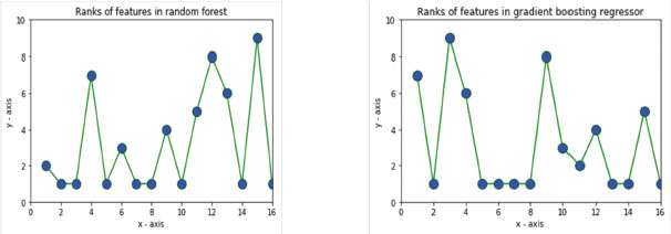
In the first phase, two tree models were used to identify and rank features and also recognized common features well. An optimal dataset was created using the best ranked features, and the mean loss and rank were calculated. Figure 2 (a) shows the analysis of the optimal dataset, with fifteen features assigned ranks using the Random Forest classifier. Figure 2 (b) displays the calculated ranks for all features using the Gradient Tree Boost classifier.

Figure 3 (a) shows the analysis of a dataset with fifteen features. The features were ranked using a Random Forest classifier with Actual Cost as the objective. Figure 3 (b) displays the ranks calculated for all the features using a Gradient Tree Boost classifier with Actual Cost as the end goal.

The experiment found that certain features were most effective in predicting the actual cost and lines of code (LOC) for RF and GTB. These features include schedule constraints, use of software tools, programmer’s capability, language experience, virtual machine experience, programming practices, application experience, turnaround time, analyst’s capability, and machine volatility. These features were found to be particularly important in estimating the actual cost.

Following the completion of the experimental research, it was discovered that the Required software reliability (rely), data base size (data), scheduling constraint (sced), Complexity of product (Time), Time constraint (Stor), Storage constraint (Acap), Virtual machine volatility (Modp), Computer turnaround time (turn), Analyst capability (LOC), Application experience (Actual Cost) attributes after feature selection and ranking and ready to prepare new optimal dataset for second phase to SDEE, On the other hand, machine volatility (virt), use of software tools (tool), virtual machine experience (vexp), found to have low significant features respectively.

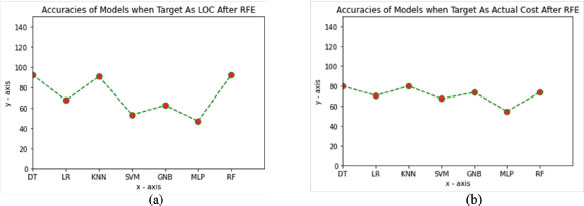
The models were evaluated using a dataset and the performance was also tested using the original dataset without extracting any features. Only the models used in the proposed stacked ensemble model were compared. The accuracy of the models varied, with Multi Layer Perception having the lowest accuracy and random forest with LOC having the highest accuracy. For the target “Actual cost,” logistic regression had the highest accuracy. The accuracy obtained by the stacked ensemble learning approach was very promising compared to the feature ranking technique, thanks to the ensemble learning algorithm’s focus on the top-ranked features.

The stacked ensemble uses different classifiers, and a graph has been created to display their performance. The x-axis represents the classifier model, while the y-axis represents the results obtained from the experiment. Figure 4 demonstrates how each model performs with and without extracting features, specifically ith the target variable being location (LOC).

The table 6 shows the performance of the high-impact features selected by RF and GTB using a separate dataset as input for the stacked ensemble. In this experiment, the target variable is actual cost and the proposed model’s accuracy is compared to other models, with the proposed stacked ensemble model showing the highest accuracy of 93.12. Similarly, the proposed stacked ensemble model also performs best with a target variable of “actual cost” at 84.05.

The below Figure 5 shows, how well each model can perform without extracting features and how well they can perform using more intense features. The Figure 5(a) and Figure 5(b) shows how well each model can perform without extracting features and target as LOC and target variable as Actual cost.

The stacked ensemble learning algorithm has shown promising accuracy compared to the feature ranking technique. This is partly because the algorithm specifically targets the top-ranked features as in Table 6.

Table 7 compares the mean absolute error and root mean square error values for different algorithms, including a proposed stacked ensemble approach. The proposed stacked ensemble had the lowest mean absolute error values compared to the other algorithms. It also had lower mean absolute error and root mean square error values when compared to all other algorithms. The values for the suggested model were 0.0227808 and 0.044150 for the ideal dataset. The results show that the proposed stacked ensemble model performed better than other base learner algorithms in terms of MAE and RMSE. In conclusion, the proposed stacked ensemble model had fewer errors than other models.

6. Conclusion

The importance of development effort estimation in creating high-quality software products cannot be disputed. Accurate estimates have evolved into a standard, challenging issue that annoys developers and clients throughout development due to software products’ Complexity and inconsistency. Cost and size are, without a mistake, the two elements that impact the evaluation of the software. It has been challenging to estimate either of these factors correctly. Even though the ensemble model is the most well-known comparison-based estimation model and has been extensively used in estimating software development efforts, it frequently fails to provide accurate estimates. A feasible approach for predicting software development efforts based on feature ranking is presented in this research, and the model’s effectiveness is proven using seven ML-based approaches. Out of the number of features considered, the simulation results show that Required software reliability (rely), database size (data), scheduling constraint (sced), Complexity of product (time), Time constraint (storage), Storage constraint (acap), Virtual machine volatility (modp), Computer turnaround time (turn), analyst capability (loc), Application experience (Actual Cost) attributes are most significant. MAE (0.0227808) and RMSE (0.044150) performance metrics were computed to assess the proposed model’s performance on the best dataset. Positive outcomes demonstrated that the proposed model can significantly improve estimation accuracy. The comparison of the obtained results with seven widely used estimation models demonstrated the superiority of the suggested models. The proposed model can only be used with prior knowledge or requirements. It is a reliable, adaptable, and flexible estimation framework, making it suitable for use in a wide range of software products, which may be used in future studies.

7. References

Abdulmajeed, A. A.; Al-Jawaherry, M. A.; Tawfeeq, T. M. 2021. Predict the required cost to develop Software Engineering projects by Using Machine Learning. In Journal of Physics: Conference Series, Conference Series (Vol. 1897, No. 1, p. 012029). IOP Publishing.

Azath, H.; Amudhavalli, P.; Rajalakshmi, S.; Marikannan, M., 2018. A novel regression neural network based optimized algorithm for software development cost and effort estimation. J. Web Eng, 17(6), 3095–3125.

Chiang, H. Y.; Lin, B. M. T., 2020. A Decision Model for Human Resource Allocation in Project Management of Software Development. IEEE Access, 8, 38073–38081. https://doi.org/10.1109/ACCESS.2020.2975829

De Carvalho, H. D. P. Fagundes, R.; Santos, W., 2021. Extreme Learning Machine Applied to Software Development Effort Estimation. IEEE Access, 9, 92676–92687. https://doi.org/10.1109/ACCESS.2021.3091313

Denard, S.; Ertas, A.; Mengel, S.; Osire, S. E., 2020. Development Cycle Modeling: Resource Estimation. MDPI-applied Science, 10, 5013. https://doi.org/10.3390/app10145013

Dewi, R. S.; Subriadi, A. P., 2017. A comparative study of software development size estimation method: UCPabc vs function points. Procedia Computer Science, 124, 470–477. https://doi.org/10.1016/j.procs.2017.12.179

Diwaker, C.; Tomar, P.; Poonia, R. C.; Singh, V. (2018). Prediction of software reliability using bio inspired soft computing techniques. Journal of medical systems, 42(5), 1–16. https://doi.org/10.1007/s10916-018-0952-3

El Bajta. M.; Idri, A., 2020. Identifying Software Cost Attributes of Software Project Management in Global Software Development: An Integrative Framework. ACM-Digital Library, 39, 1–5. https://doi.org/10.1145/3419604.3419780

Ghatasheh, N.; Faris, H.; Aljarah, I.; Al-Sayyed, R. M., 2019. Optimizing software effort estimation models using firefly algorithm. arXiv preprint arXiv:1903.02079.

Hai, V. V.; Nhung, H. L. T. K., Prokopova, Z.; Silhavy, R.; Silhavy, P., 2021. A New Approach to Calibrating Functional Complexity Weight in Software Development Effort Estimation. MDPI-Computers, 11(2). https://doi.org/10.3390/computers11020015

Hasan, M. A. M.; Nasser, M.; Ahmad, S.; Molla, K. I. (2016). Feature selection for intrusion detection using random forest. Journal of information security, 7(3), 129–140. https://doi.org/10.4236/jis.2016.73009

Idri, A.; Abran, A.; Khoshgoftaar, T. M., 2002, June. Estimating software project effort by analogy based on linguistic values. Proceedings Eighth IEEE Symposium on Software Metrics (pp. 21–30). IEEE

Jing, X. Y.; Qi, F.; Wu, F.; Xu, B., 2016, May. Missing data imputation based on low-rank recovery and semi-supervised regression for software effort estimation. 2016 IEEE/ACM 38th International Conference on Software Engineering (ICSE) (pp. 607–618). IEEE. https://doi.org/10.1145/2884781.2884827

Kuhail; M. A.; Lauesen, S., 2022. User Story Quality in Practice: A Case Study. MDPI-Software, 1, 223–243. https://doi.org/10.3390/software1030010

Kumar, K.; Aihole, S.; Putage, S., 2017. Anticipation of software development effort using artificial neural network for NASA data sets. Int J Eng Sci, 7(5), 11228.

Mak, L.; Taheri, P., 2022. An Automated Tool for Upgrading Fortran Codes. MDPI-Software, 1, 299–315, 2022. doi: https://doi.org/10.3390/software1030014

Mashkoor, A.; Menzies, T.; Egyed, A.; Ramler, R., 2022. Artificial Intelligence and Software Engineering: Are We Ready? Computer, 55(3), 24–28. https://doi.org/10.1109/MC.2022.3144805

Mensah, S.; Keung, J.; Bosu, M. F.; Bennin, K. E., 2018. Duplex output software effort estimation model with self-guided interpretation. Information and Software Technology, 94, 1–13. https://doi.org/10.1016/j.infsof.2017.09.010

Menzies, T.; Yang, Y.; Mathew, G.; Boehm, B.; Hihn, J., 2017. Negative results for software effort estimation. Empirical Software Engineering, 22(5), 2658–2683. https://doi.org/10.1007/s10664-016-9472-2

Mustapha, H.; Abdelwahed, N., 2019. Investigating the use of random forest in software effort estimation. Procedia computer science, 148, 343–352. https://doi.org/10.1016/j.procs.2019.01.042

Nassif, A. B.; Azzeh, M.; Idri, A.; Abran, A., 2019. Software development effort estimation using regression fuzzy models. Computational intelligence and neuroscience. https://doi.org/10.1155/2019/8367214

Phannachitta, P.; Keung, J.; Monden, A.; Matsumoto, K., 2017. A stability assessment of solution adaptation techniques for analogy-based software effort estimation. Empirical Software Engineering, 22(1), 474–504. https://doi.org/10.1007/s10664-016-9434-8

Pillai, K.; Jeyakumar, M., 2019. A real time extreme learning machine for software development effort estimation. Int. Arab J. Inf. Technol., 16(1), 17–22.

Pospieszny, P.; Czarnacka-Chrobot, B.; Kobylinski, A., 2018. An effective approach for software project effort and duration estimation with machine learning algorithms. Journal of Systems and Software, 137, 184–196. https://doi.org/10.1016/j.jss.2017.11.066

Rani, P.; Kumar, R.; Jain, A.; Chawla, S. K., 2021. A hybrid approach for feature selection based on genetic algorithm and recursive feature elimination. International Journal of Information System Modeling and Design (IJISMD), 12(2), 17–38. https://doi.org/10.4018/IJISMD.2021040102

Rao, K. E.; Rao, G. A., 2021. Ensemble learning with recursive feature elimination integrated software effort estimation: a novel approach. Evolutionary Intelligence, 14(1), 151–162. https://doi.org/10.1007/s12065-020-00360-5

Rijwani, P.; Jain, S., 2016. Enhanced software effort estimation using multi layered feed forward artificial neural network technique. Procedia Computer Science, 89, 307–312. https://doi.org/10.1016/j.procs.2016.06.073

Rosen, C. 2020. Guide to Software Systems Development-Connecting Novel Theory and Current Practice. Springer International Publishing. https://doi.org/10.1007/978-3-030-39730-2

Shah, J.; Kama, N., 2018, February. Extending function point analysis effort estimation method for software development phase. In Proceedings of the 2018 7th International Conference on Software and Computer Applications (pp. 77–81). https://doi.org/10.1145/3185089.3185137

Singh, C.; Sharma, N.; Kumar, N., 2019. An Efficient Approach for Software Maintenance Effort Estimation Using Particle Swarm Optimization Technique. International Journal of Recent Technology and Engineering (IJRTE), 7(6C).

V.V. Hai, H.L.T.K. Nhung, Z. Prokopova, R. Silhavy, P. Silhavy, 2021. A New Approach to Calibrating Functional Complexity Weight in Software Development Effort Estimation, MDPI-Computers, vol.11, No.2. https://doi.org/10.3390/computers11020015