
Figure 1. Nonlinear model of a neuron (a) and transfer function (b)
Comparison of Swarm-based Metaheuristic and Gradient Descent-based Algorithms in Artificial Neural Network Training
Erdal Ekera, Murat Kayrib, Serdar Ekincic, and Davut İzcic, d
a Vocational School of Social Sciences, Muş Alparslan University, Muş, Turkey
b Department of Computer and Instructional Technology Education, Van Yüzüncü Yıl University, Van, Turkey
c Department of Computer Engineering, Batman University, Batman, Turkey
d MEU Research Unit, Middle East University, Amman, Jordan
e.eker@alparslan.edu.tr, muratkayri@yyu.edu.tr, serdar.ekinci@batman.edu.tr, davut.izci@batman.edu.tr
ABSTRACT
This paper aims to compare the gradient descent-based algorithms under classical training model and swarm-based metaheuristic algorithms in feed forward backpropagation artificial neural network training. Batch weight and bias rule, Bayesian regularization, cyclical weight and bias rule and Levenberg-Marquardt algorithms are used as the classical gradient descent-based algorithms. In terms of the swarm-based metaheuristic algorithms, hunger games search, gray wolf optimizer, Archimedes optimization, and the Aquila optimizer are adopted. The Iris data set is used in this paper for the training. Mean square error, mean absolute error and determination coefficient are used as statistical measurement techniques to determine the effect of the network architecture and the adopted training algorithm. The metaheuristic algorithms are shown to have superior capability over the gradient descent-based algorithms in terms of artificial neural network training. In addition to their success in error rates, the classification capabilities of the metaheuristic algorithms are also observed to be in the range of 94%-97%. The hunger games search algorithm is also observed for its specific advantages amongst the metaheuristic algorithms as it maintains good performance in terms of classification ability and other statistical measurements.
KEYWORDS
classification; swarm-based metaheuristic algorithms; gradient descentbased algorithm; artificial neural networks
1. Introduction
Artificial neural networks can be trained to approximate almost any smooth, measurable function (Hornik et al., 1989), thus, they can model high-dimensional nonlinear functions without making preliminary estimations. Thanks to this feature, artificial neural networks can be trained to correctly classify different data sets and it makes them preferable over other techniques (Nguyen et al., 2021, Jawad et al., 2021). This paper considers the preferability of ANNs and determines the most convenient training strategy by looking at strategies based on swarm-based metaheuristic and gradient descent-based algorithms.
Classical methods have many disadvantages e.g., difficulties in finding suitable artificial neural network architectures and being unable to reach global optimum values (Ghaffari et al., 2006). Unlike classical methods, metaheuristic algorithms have the ability to avoid local optimum points and reach the global optimum point in the shortest time (Eker et al., 2021). Therefore, the use of metaheuristic approaches as supervised algorithms has also become preferable in addition to the classical methods (Heidari et al., 2019). For example, metaheuristic approaches such as genetic algorithm, biogeography-based optimizer, particle swarm optimization, cuckoo search, firefly algorithm, artificial bee colony algorithm and simulated annealing have been used for training neural networks adopted to industrial applications (Chong et al., 2021, Ly et al., 2021). Likewise, chicken swarm optimization (Khan et al., 2019), chimp optimization algorithm (Khishe et al., 2019), sperm whale algorithm (Engy et al., 2018) have been employed to solve real world problems with artificial neural networks. For more examples of swarm-based metaheuristic algorithms developed in recent years, the readers are referred to the work conducted by (Dragoi et al., 2021).
This paper takes the good capability of metaheuristic techniques into account and aims to provide a comparative assessment between gradient descent-based algorithms and some of the well performing swarm-based metaheuristic algorithms in order to provide a new and a wider perspective on the previous attempts, showing different comparative assessments (Devikanniga et al., 2019; Ray, 2019). In this regard, batch weight and bias rule (Grippo, 2000), Bayesian regularization (Wang et al., 2007), Levenberg-Marquardt (Wang et al., 2007) and cyclical weight and bias rule (Shabani and Mazahery, 2012) algorithms are adopted as gradient descent-based techniques for this work. Likewise, hunger games search algorithm (Yang et al., 2021), grey wolf optimizer (Mirjalili et al., 2014), Archimedes optimization algorithm (Hashim et al., 2021) and Aquila optimizer (Abualigah et al., 2021) are used as metaheuristic approaches for comparative assessments. Several statistical metrics have been used in the comparative study and evidence that metaheuristic approaches perform better in artificial neural network training. Then, the most efficient swarm-based metaheuristic approach is identified through classical and CEC2017 benchmark functions.
The rest of the paper is organized as follows. The section that follows explains the artificial neural networks and the respective training algorithms. In section three, the statistical results achieved by the training algorithms are presented. Section four is dedicated to the assessment of the classification abilities of the swarm-based metaheuristic techniques and demonstrates that highest efficiency has been achieved by the hunger games search algorithm. Finally, the paper is concluded in section five.
2. Artificial Neural Networks
Artificial neural networks (ANNs) have an architecture that simulates the human brain’s information processing structure. This architecture accumulates, generalizes, and finalizes the information presented to it with the connection weights of many nodes consisting of different phases (Haykin, 2005). Figure 1 presents the nonlinear model of a neuron and transfer function adopted in an ANN structure. The mathematical model of a k node is expressed in the following forms:
Figure 1. Nonlinear model of a neuron (a) and transfer function (b)
where x1,x2,…,xm are input signals, w_(k1),wk2,…,wkm are synaptic weights of node k, uk is the input signal, bk is the bias, φ(.) is the activation function, yk is the output signal, and vk is the activation potential of node k. vk and yk are defined as follows.
Logistic (logsig) function is a type of sigmoid function that is used as an activation function in ANN. It is defined as follows where α is the slope parameter of the sigmoid function.
The way a neural network's nodes are structured is closely linked to the learning algorithm used to train the network. Different network architectures require appropriate learning algorithms. For this reason, the structure of neural networks also determines which learning algorithm will be used. Multilayer perceptron is used in this paper (Lv and Qiao, 2020). This structure has a hidden layer that includes computation nodes (Gardner and Dorling,1998). For more detailed background information on this model, the readers are referred to the work carried out by (Hecht-Nielsen, 1992).
2.1. ANN Training
There are two types of learning methods for ANNs. First method is an unsupervised learning method which is used for clustering the data. The second type is supervised learning method which is used for classifying the data. This paper adopts the supervised learning method (Movassagh, 2021). The iris dataset is used for training the ANN with the selected algorithms (Fisher, 1936). This dataset consists of three classes, two of which are not linearly separable, and contains 150 data samples with 4 continuous input variables. There are available training algorithms that optimize the ANN. The selection of the algorithms is important in order to obtain the best result (Gupta and Raza, 2019). In this context, this paper uses gradient descent and swarm-based metaheuristics algorithms to train the ANN. Figure 2 shows how an algorithm is used for the optimization process of the ANN training.

Figure 2. Flowchart of the optimization process of the ANN training
2.2. ANN Training Algorithms
Training processes usually consist of mounting the database used for training, creating the network architecture, training the network, and simulating the network's response to new inputs. Two strategies of the back propagation algorithm, which has many variations, are studied in this paper. The first four algorithms are gradient descent-based algorithms (Paulin and Santhakumaran, 2011; Sönmez, 2018) and presented in the following subsection whereas the next four ones are swarm-based metaheuristic algorithms (Gupta and Raza, 2019, Eker et al., 2021) presented in subsection 2.2.2.
2.2.1. Gradient Descent-Based Algorithms
Optimizing the weights in the ANN is the key to modelling the classification correctly. However, adjusting the weights depends on adjusting the gradient descent weights and the direction of change of slope during backpropagation. Many optimization algorithms have been proposed in recent years to avoid the problems of stagnating the local minimum as well as the curse of dimensionality. The best-known gradient descent optimization algorithms can be listed as batch weight and bias rule, Bayesian regularization, Levenberg-Marquardt and cyclical weight and bias rule (Dogo et al., 2018).
Batch weight and bias rule (B) algorithm updates each weight and bias values according to the learning function after each cycle, and the training is completed when the maximum iteration is reached, or the performance of the verification data reaches the specified value (Grippo, 2000). The Bayesian regularization (BR) algorithm, on the other hand, is a traditional way of dealing with the negative effect of large weights. The idea of regularization is to make the network response smoother through modification in the objective function by adding a penalty term that consists of the squares of all network weights. In this strategy, the weight and bias values are updated according to the Levenberg-Marquardt (LM) optimization. The working method is to minimize the combination of squares of error and weight, called Bayesian regularization, and then determine the right combination to form a well generalizing network (Wang et al., 2007). In the cyclical weight and bias rule (C) algorithm, the inputs are sequential and at each iteration, each data vector is presented to the network, updating the weights and biases (Shabani and Mazahery, 2012).
2.2.2. Swarm-Based Metaheuristic Algorithms
This group of algorithms have attracted attention due to their flexible and simple structure along with the ability to avoid local optimum. The metaheuristic algorithms consider any given problem as a black box, and they attempt to solve it regardless of its nature. Therefore, metaheuristic algorithms can easily be applied to any real-world problem (Eker et al., 2021). For more details on the training of ANN with metaheuristic algorithms, the readers are referred to the work of (Devikanniga et al., 2019). The research presented this paper adopted hunger games search (HGS) algorithm, grey wolf optimizer (GWO), Archimedes optimization algorithm (AOA) and the Aquila optimizer (AO) as swarm-based metaheuristic algorithms.
The HGS algorithm designs and uses an adaptive weight based on the concept of hunger and simulates the effect of hunger at each search step (Yang et al., 2021). It follows the computable games used by almost all animals. These competitive games have adaptive evolutionary character and ensure the survival of animals. The GWO algorithm, on the other hand, is inspired by the behavior of the grey wolf swarm (Mirjalili et al., 2014). It mimics the leadership structure and hunting mechanism of the swarm by applying different strategies called hunting, seeking, siege and attacking. Unlike the latter described metaheuristics, the AOA algorithm is inspired from the Archimedes' law, known as the buoyancy of water (Hashim et al., 2021). This algorithm mimics what happens when objects of different weights and volumes are immersed in a liquid. The last swarm-based metaheuristic algorithm used in this paper is the AO algorithm which is inspired by the Aquila's foraging behavior in nature (Abualigah et al., 2021). The optimization procedure of the AO algorithm is represented with four steps: selecting a high glide search space with vertical stoop, exploring a diverging search space with a short glide attack by contour flight, using a low flight convergence search space with a slow descent attack and gliding by walking and catching prey.
For all the adopted algorithms, the default parameter settings are used which were reported in the respective original publications (Yang et al., 2021; Mirjalili et al., 2014; Hashim et al., 2021; Abualigah et al., 2021). The detailed procedures and flowcharts of those algorithms can also be found in those studies. The related details are not included in this paper in order to avoid unnecessary background information.
3. Experimental Results
In ANN training, errors occur between the output values and the desired output values of the training algorithm. The aim of the error metric is to measure the performance of the ANN (Eren et al., 2016). The errors that are closer to 0 mean that the optimization of the network is better. To calculate the error values, mean square error (MSE), mean absolute error (MAE) and determination coefficient (R2), can be used. These functions are defined as follows (Kayri, 2015; Mirjalili, 2015):
where, i is input unit, Pi is desired and Oi is the observed values, is mean desired value, and N is the number of outputs. For the training of gradient descent-based algorithms, 500 epochs were used in this work whereas for the metaheuristic algorithms, 500 iterations and 40 search agents were adopted. For both strategies, 30 independent runs were carried out by using MATLAB software. Table 1 presents the comparative results of the adopted algorithms in terms of MSE, MAE and R2 values. In Table 1, it is observed that the swarm-based metaheuristic algorithms have been more successful, especially the HGS algorithm which had low values in error rates and a closeness between the expected and observed results in ANN training (R2 = 95%). The boxplots provided in Figure 3 offer an illustrative appreciation. The closeness of the median to the desired fit value in the algorithms shows the superiority of swarm-based metaheuristic algorithms.
Table 1. Comparative MSE, MAE and R2values calculated for different algorithms
|
Optimizer |
Strategies |
Metric |
Logsig |
Rank of each metrics |
FEED-FORWARD ARTIFICIAL BACKPROPAGATION NETWORKS |
GRADIENT DESCENT-BASED ALGORITHMS |
B |
Best MSE |
0.6990 |
8 |
Best MAE |
0.6737 |
8 |
|||
R2 |
0.6550 |
4 |
|||
BR |
Best MSE |
0.3800 |
6 |
||
Best MAE |
0.4104 |
6 |
|||
R2 |
0.6329 |
5 |
|||
C |
Best MSE |
0.4324 |
7 |
||
Best MAE |
0.4712 |
7 |
|||
R2 |
0.3325 |
6 |
|||
LM |
Best MSE |
0.3565 |
5 |
||
Best MAE |
0.3833 |
5 |
|||
R2 |
0.7560 |
3 |
|||
SWARM-BASED METAHEURISTIC ALGORITHMS |
HGS |
Best MSE |
0.0133 |
1 |
|
Best MAE |
0.0180 |
1 |
|||
R2 |
0.9500 |
1 |
|||
GWO |
Best MSE |
0.0242 |
3 |
||
Best MAE |
0.0237 |
2 |
|||
R2 |
0.9500 |
1 |
|||
AOA |
Best MSE |
0.3291 |
4 |
||
Best MAE |
0.3344 |
4 |
|||
R2 |
0.9400 |
2 |
|||
AO |
Best MSE |
0.0177 |
2 |
||
Best MAE |
0.0237 |
3 |
|||
R2 |
0.9500 |
1 |
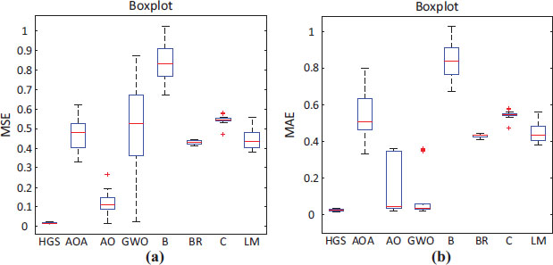
Figure 3. Boxplots of MSE (a) and MAE (b) values obtained with different algorithms
The convergence curves presented in Figure 4 prove the superiority of the swarm-based metaheuristic algorithms as they converge to the lowest values indicating their ability to avoid local minimum stagnation. The convergence curves also show that the HGS algorithm specifically has a fast tendency to avoid the stagnation problem. Considering the results presented in the respective table and figures, the swarm-based metaheuristic algorithms can be described as the more convenient and advantageous structures compared to the classical algorithms.
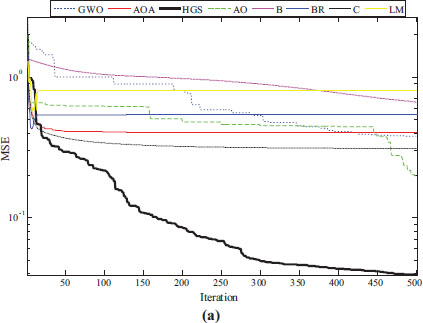
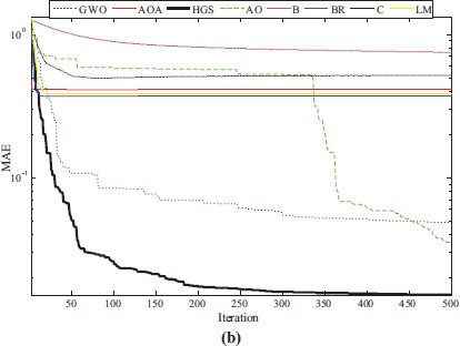
Figure 4. Convergence curves with respect to MSE (a) and MAE (b) values
4. Determination of the Best Metaheuristics for ANN Training
Having lower error rates is an indication of superiority of the swarm-based metaheuristic algorithms over the gradient descent-based algorithms in terms of ANN training strategies. Therefore, this section investigates the most suitable metaheuristic algorithm by adopting different benchmark functions. Specifically, the superiority of the HGS algorithm is demonstrated. In this regard, well-known twenty-three classical (unimodal, multimodal, and low dimensional) and twenty-nine CEC2017 benchmark functions have been adopted. It is worth noting that C2 test function from CEC2017 test suite has been removed from this paper as it has an unstable structure (Mohamed et al., 2020).
4.1. Classification Success
After training a model, confusion matrix is used to measure performance for each class separately. This matrix also helps identify areas where a classification algorithm performs poorly. In the graph presented in Figure 5, the rows show the actual class, while the columns show the predicted class.
Figure 5. Classification rates of swarm-based metaheuristic algorithms
In here, the true positive rate (TPR) and false negative rate (FNR) indicators present the true and misclassified rates of observations. The superior performance of the HGS algorithm can be observed from Figure 5. The numerical classification results presented in Table 2 further confirm the superior classification capability of the HGS algorithm over the other swarm-based metaheuristic algorithms.
Table 2. Results of the classifications
Transfer function |
Arrangement |
Algorithms |
|||
HGS |
GWO |
AOA |
AO |
||
Logsig |
Mean Classification (%) |
96.70 |
94.70 |
95.30 |
94.70 |
Rank |
1 |
3 |
2 |
3 |
|
4.2. Performance Assessment on Different Benchmarks
This paper further assesses the performance of the swarm-based metaheuristic algorithms on different benchmark sets. The first set consisted of well-known twenty-three classical benchmark functions which are presented in Table 3. Further assessments have also been carried out using the twenty-nine benchmark functions from the challenging CEC2017 test suite listed in Table 4.
Table 3. Adopted classical benchmark functions
Function type and name |
Dimension |
Range |
Optimum |
|
Unimodal function |
||||
F1 |
Sphere |
30 |
[−100,100] |
0 |
F2 |
Schwefel 2.2 |
30 |
[−10,10] |
0 |
F3 |
Schwefel 1.2 |
30 |
[−100,100] |
0 |
F4 |
Schwefel 2.21 |
30 |
[−100,100] |
0 |
F5 |
Rosenbrock |
30 |
[−30,30] |
0 |
F6 |
Step |
30 |
[−100,100] |
0 |
F7 |
Quartic |
30 |
[−1.28,1.28] |
0 |
Multimodal function |
||||
F8 |
Schwefel |
30 |
[−500,500] |
-1.2569E+04 |
F9 |
Rastrigin |
30 |
[−5.12,5.12] |
0 |
F10 |
Ackley |
30 |
[−32,32] |
0 |
F11 |
Griewank |
30 |
[−600,600] |
0 |
F12 |
Penalized |
30 |
[−50,50] |
0 |
F13 |
Penalized2 |
30 |
[−50,50] |
0 |
Low-dimensional function |
||||
F14 |
Foxholes |
2 |
[−65.536,65.536] |
0.998 |
F15 |
Kowalik |
4 |
[−5,5] |
3.0749E−04 |
F16 |
Six-Hump Camel |
2 |
[−5,5] |
-1.0316 |
F17 |
Branin |
2 |
[−5,10]×[0,15] |
0.39789 |
F18 |
Goldstein-Price |
2 |
[−2,2] |
3 |
F19 |
Hartman 3 |
3 |
[0,1] |
-3.8628 |
F20 |
Hartman 6 |
6 |
[0,1] |
-3.322 |
F21 |
Shekel 5 |
4 |
[0,10] |
-10.1532 |
F22 |
Shekel 7 |
4 |
[0,10] |
-10.4029 |
F23 |
Shekel 10 |
4 |
[0,10] |
-10.5364 |
Table 4. Adopted CEC2017 benchmark functions
Function type and name |
Range |
Dimension |
Optimum |
|
Shifted and rotated function |
||||
C1 |
Bent Cigar function |
[−100,100] |
30 |
100 |
C2 |
Sum of differential power function |
[−100,100] |
30 |
200 |
C3 |
Zakharov function |
[−100,100] |
30 |
300 |
C4 |
Rosenbrock’s function |
[−100,100] |
30 |
400 |
C5 |
Rastrigin’s function |
[−100,100] |
30 |
500 |
C6 |
Expanded Schaffer’s F6 function |
[−100,100] |
30 |
600 |
C7 |
Lunacek Bi-Rastrigin function |
[−100,100] |
30 |
700 |
C8 |
Non-continuous Rastrigin’s function |
[−100,100] |
30 |
800 |
C9 |
Levy function |
[−100,100] |
30 |
900 |
C10 |
Schwefel’s function |
[−100,100] |
30 |
1000 |
Hybrid function |
||||
C11 |
Function 1 (N = 3) |
[−100,100] |
30 |
1100 |
C12 |
Function 2 (N = 3) |
[−100,100] |
30 |
1200 |
C13 |
Function 3 (N = 3) |
[−100,100] |
30 |
1300 |
C14 |
Function 4 (N = 4) |
[−100,100] |
30 |
1400 |
C15 |
Function 5 (N = 4) |
[−100,100] |
30 |
1500 |
C16 |
Function 6 (N = 4) |
[−100,100] |
30 |
1600 |
C17 |
Function 6 (N = 5) |
[−100,100] |
30 |
1700 |
C18 |
Function 6 (N = 5) |
[−100,100] |
30 |
1800 |
C19 |
Function 6 (N = 5) |
[−100,100] |
30 |
1900 |
C20 |
Function 6 (N = 6) |
[−100,100] |
30 |
2000 |
Composition function |
||||
C21 |
Function 1 (N = 3) |
[−100,100] |
30 |
2100 |
C22 |
Function 2 (N = 3) |
[−100,100] |
30 |
2200 |
C23 |
Function 3 (N = 4) |
[−100,100] |
30 |
2300 |
C24 |
Function 4 (N = 4) |
[−100,100] |
30 |
2400 |
C25 |
Function 5 (N = 5) |
[−100,100] |
30 |
2500 |
C26 |
Function 6 (N = 5) |
[−100,100] |
30 |
2600 |
C27 |
Function 7 (N = 6) |
[−100,100] |
30 |
2700 |
C28 |
Function 8 (N = 6) |
[−100,100] |
30 |
2800 |
C29 |
Function 9 (N = 3) |
[−100,100] |
30 |
2900 |
C30 |
Function 10 (N = 3) |
[−100,100] |
30 |
3000 |
In classical test functions listed in Table 3, F1-F7 have the unimodal features and are appropriate for testing the exploitation abilities of the algorithms. On the other hand, F8-F13 are multimodal test functions and can be used for the evaluation of the exploration, whereas F14-F23 are low and fixed dimensional test functions that can be used to test the solution quality of the algorithms.
The results of the classical test functions are presented in Table 5. F1-F23 demonstrate the competitive structures of the swarm-based metaheuristic algorithms. However, the HGS algorithm demonstrates an overall superior capability. Apart from the test functions of F5 and F7, the HGS algorithm finds more excellent solutions compared to the other swarm-based metaheuristic algorithms. The good capability of the HGS algorithm can also be observed from the convergence curves presented in Fig. 6.
Table 5. Statistical results for classical test functions
Function Name |
Measurement Tools |
HGS |
AOA |
AO |
GWO |
F1 |
Best |
0.000E+00 |
2.6209E−229 |
2.8890E−164 |
2.2865E−32 |
Worst |
0.000E+00 |
6.0532E−40 |
1.1504E−108 |
3.2161E−30 |
|
Std. Dev. |
0.000E+00 |
1.1052E−40 |
2.1003E−109 |
8.0191E−31 |
|
Average time |
0.1349 |
0.1664 |
0.3304 |
0.2332 |
|
F2 |
Best |
0.000E+00 |
0.000E+00 |
7.0922E−84 |
3.2726E−19 |
Worst |
2.2102E−87 |
0.000E+00 |
9.8074E−57 |
5.0220E−18 |
|
Std. Dev. |
4.0352E−88 |
0.000E+00 |
1.7906E−57 |
8.9698E−19 |
|
Average time |
0.1395 |
0.1687 |
0.3047 |
0.2271 |
|
F3 |
Best |
0.000E+00 |
5.2200E−144 |
1.5738E−164 |
8.7926E−10 |
Worst |
3.9925E−90 |
1.8200E−02 |
2.9484E−103 |
1.3183E−05 |
|
Std. Dev. |
7.3070E−91 |
5.9000E−03 |
5.3824E−104 |
2.5832E−06 |
|
Average time |
0.4944 |
0.4460 |
0.9330 |
0.5267 |
|
F4 |
Best |
0.000E+00 |
6.2997E−89 |
8.1998E−83 |
2.0183E−08 |
Worst |
5.8285E−88 |
5.4700E−02 |
3.1755E−67 |
2.9897E−07 |
|
Std. Dev. |
1.0638E−88 |
2.0000E−2 |
5.7945E−68 |
6.9925E−08 |
|
Average time |
0.1395 |
0.1580 |
0.3237 |
0.2365 |
|
F5 |
Best |
1.5468E−04 |
27.2557 |
8.8710E−06 |
25.5570 |
Worst |
2.5199E+01 |
2.8938E+01 |
3.1800E−02 |
2.8550E+01 |
|
Std. Dev. |
1.2544E+01 |
3.7560E−01 |
5.8000E−03 |
7.326E−01 |
|
Average time |
0.1721 |
0.1874 |
0.3882 |
0.2548 |
|
F6 |
Best |
6.4838E−09 |
2.2032E+00 |
3.2297E−07 |
3.4546E−05 |
Worst |
3.5290E−05 |
3.3972E+00 |
1.7995E−04 |
9.9280E−01 |
|
Std. Dev. |
7.0923E−06 |
3.1640E−01 |
4.1202E−05 |
2.4800E−01 |
|
Average time |
0.106 |
0.095 |
0.2035 |
0.1469 |
|
F7 |
Best |
2.7724E−05 |
2.2815E−06 |
2.3947E−06 |
5.5999E−04 |
Worst |
4.1000E−03 |
1.9606E−04 |
2.4662E−04 |
3.6000E−03 |
|
Std. Dev. |
1.000E−03 |
4.3839E−05 |
6.3789E−05 |
7.6880E−04 |
|
Average time |
0.1806 |
0.1811 |
0.3736 |
0.2344 |
|
F8 |
Best |
−1.2569E+04 |
-6.3161E+03 |
-1.2566E+04 |
-7.8919E+03 |
Worst |
-1.2569E+04 |
-4.2969E+03 |
-3.8545E+03 |
-3.3883E+03 |
|
Std. Dev. |
9.941E−01 |
3.9623E+02 |
3.8947E+03 |
1.0701E+03 |
|
Average time |
0.1149 |
0.1152 |
0.2488 |
0.1653 |
|
F9 |
Best |
0.000E+00 |
0.000E+00 |
0.000E+00 |
0.000E+00 |
Worst |
0.000E+00 |
0.000E+00 |
0.000E+00 |
1.4747 E+01 |
|
Std. Dev. |
0.000E+00 |
0.000E+00 |
0.000E+00 |
4.0251E+00 |
|
Average time |
0.0116 |
0.0200 |
0.3109 |
0.2182 |
|
F10 |
Best |
8.8818E−16 |
8.8818E−16 |
8.8818E−16 |
4.4409E−15 |
Worst |
8.8818E−16 |
8.8818E−16 |
8.8818E−16 |
7.9936E−15 |
|
Std. Dev. |
1.0029E−31 |
1.0029E−31 |
1.0029E−31 |
1.5979E−15 |
|
Average time |
0.0051 |
0.1000 |
0.2511 |
0.1172 |
|
F11 |
Best |
0.000E+00 |
4.8000E−03 |
0.000E+00 |
0.000E+00 |
Worst |
0.000E+00 |
0.5223 |
0.000E+00 |
2.4802E−02 |
|
Std. Dev. |
0.000E+00 |
0.1074 |
0.000E+00 |
7.7011E−03 |
|
Average time |
0.012 |
0.1742 |
0.3843 |
0.2479 |
|
F12 |
Best |
1.6561E−10 |
3.5810E−01 |
1.3848E−08 |
9.9246E−06 |
Worst |
1.3959 E−07 |
5.4980E−01 |
8.9249E−06 |
8.5402E−02 |
|
Std. Dev. |
3.1648 E−08 |
5.1701E−02 |
2.4732E−06 |
1.7200E−03 |
|
Average time |
0.0170 |
0.5203 |
1.0472 |
0.5973 |
|
F13 |
Best |
4.5870E−09 |
2.5985E+00 |
9.6151E−11 |
1.0610E−01 |
Worst |
5.3853E−06 |
2.9944E+00 |
2.0452E−04 |
9.4680E−01 |
|
Std. Dev. |
1.1118E−06 |
9.2003E−01 |
4.0636E−05 |
2.0961E−01 |
|
Average time |
0.0169 |
0.5146 |
1.0235 |
0.5901 |
|
F14 |
Best |
9.9800 E−01 |
9.9800E−01 |
9.9800E−01 |
9.9800E−01 |
Worst |
9.9800E−01 |
1.2671E+01 |
1.2671E+01 |
1.2671E+01 |
|
Std. Dev. |
3.3876E−16 |
4.5595E+00 |
2.7180E+00 |
4.3051E+00 |
|
Average time |
0.0298 |
0.9223 |
1.9254 |
0.9192 |
|
F15 |
Best |
3.0749E−04 |
3.4417E−04 |
3.2317E−04 |
3.0750E−04 |
Worst |
1.2001E−03 |
1.1030E−01 |
8.7196E−04 |
2.0400E−02 |
|
Std. Dev. |
2.3278E−04 |
3.3603E−02 |
1.1782E−04 |
6.9012E−03 |
|
Average time |
0.0807 |
0.0940 |
0.2312 |
0.2313 |
|
F16 |
Best |
−1.0316E+00 |
−1.0316E+00 |
−1.0316E+00 |
−1.0316E+00 |
Worst |
−1.0316E+00 |
−1.0316E+00 |
-1.0304E+00 |
−1.0316E+00 |
|
Std. Dev. |
0.000E+00 |
1.1764E−07 |
2.7520E−04 |
3.1617E−08 |
|
Average time |
0.0715 |
0.0828 |
0.2095 |
0.0861 |
|
F17 |
Best |
3.9790E−01 |
0.3980 |
3.9790E−01 |
3.9790E−01 |
Worst |
3.9790E−01 |
0.4390 |
3.9790E−01 |
3.9790E−01 |
|
Std. Dev. |
1.1292E−16 |
8.1000E−03 |
2.2853E−04 |
1.3893E−06 |
|
Average time |
0.0735 |
0.0782 |
0.2057 |
0.0745 |
|
F18 |
Best |
3.0000E+00 |
3.0000E+00 |
3.0043E+00 |
3.0000E+00 |
Worst |
3.0000E+00 |
9.2879E+01 |
3.0825E+00 |
3.0001E+00 |
|
Std. Dev. |
3.7790E−15 |
1.9427E+01 |
2.6300E+02 |
2.9345E−05 |
|
Average time |
0.0587 |
0.0671 |
0.1980 |
0.0730 |
|
F19 |
Best |
−3.8628E+00 |
-3.8587E+00 |
−3.8628E+00 |
−3.8628E+00 |
Worst |
−3.8628E+00 |
-3.8445E+00 |
-3.8480E+00 |
−3.8628E+00 |
|
Std. Dev. |
2.7101E−15 |
0.0034 |
0.0034 |
0.0027 |
|
Average time |
0.0863 |
0.0953 |
0.2439 |
0.1006 |
|
F20 |
Best |
−3.3220E+00 |
-3.2170 E+00 |
-3.3148 E+00 |
−3.3220E+00 |
Worst |
−3.2031E+00 |
-3.0612E+00 |
-2.8523E+00 |
-3.1352E+00 |
|
Std. Dev. |
5.9200 E+00 |
3.4400E−02 |
1.0120E−01 |
7.5401E−02 |
|
Average time |
0.0924 |
0.0326 |
0.2614 |
0.1135 |
|
F21 |
Best |
−1.0153E+01 |
-6.8444E+00 |
−1.0153E+01 |
-1.0152E+01 |
Worst |
-5.0552E+00 |
-1.9030E+00 |
−1.0094E+01 |
-5.0552E+00 |
|
Std. Dev. |
1.2934E+00 |
1.2022E+00 |
1.2900E−02 |
1.2873E+00 |
|
Average time |
0.1001 |
0.1201 |
0.2826 |
0.1179 |
|
F22 |
Best |
−1.0403E+01 |
-6.9925 |
-1.0402E+01 |
-1.0402E+01 |
Worst |
-5.0877E+00 |
-1.8047E+00 |
-1.0380E+01 |
-5.1269E+00 |
|
Std. Dev. |
1.3485E+00 |
1.0643E+00 |
6.0000E−03 |
9.6290E+01 |
|
Average time |
0.1115 |
0.1215 |
0.2883 |
0.1332 |
|
F23 |
Best |
−1.0536E+01 |
-8.2004E+00 |
-1.0536E+01 |
-1.0536E+01 |
Worst |
-5.1285E+00 |
-1.7588E+00 |
−1.0503E+01 |
-2.4216E+00 |
|
Std. Dev. |
9.8730E−01 |
1.5005E+00 |
8.4000E−03 |
2.2382E+00 |
|
Average time |
0.1302 |
0.1464 |
0.3343 |
0.1506 |

Figure 6. Comparative convergence curves for some of the classical benchmark functions
The results related to CEC2017 test functions are presented in Table 6. In terms of the challenging functions from the CEC2017 test suite, the HGS algorithm demonstrates the ability to find solutions in the shortest time. This can also be observed from the convergence curves presented in Figure 7. In terms of the optimizing ability, the HGS also achieves the best score in most of the test functions, indicating its excellent capability.
Table 6. The obtained results from CEC2017 test suite
Function Name |
Measurement Tools |
HGS |
AOA |
AO |
GWO |
C1 |
Best |
7.0667E+03 |
3.3891E+10 |
7.8392E+05 |
3.8885E+08 |
Worst |
9.5968E+07 |
7.3225E+10 |
3.1294E+06 |
5.6049E+09 |
|
Std. Dev. |
2.3974E+07 |
1.0034E+10 |
6.2190E+05 |
1.6846E+09 |
|
Average time |
0.1544 |
0.1545 |
1.8225 |
0.2277 |
|
C3 |
Best |
1.5875E+04 |
4.4288E+04 |
1.4829E+04 |
3.2442E+04 |
Worst |
9.0101E+04 |
9.3836E+04 |
3.7164E+04 |
7.7307E+04 |
|
Std. Dev. |
1.8329E+04 |
1.0697E+04 |
4.6219E+03 |
1.1986E+04 |
|
Average time |
0.1578 |
0.1651 |
1.8191 |
0.2225 |
|
C4 |
Best |
4.3618E+02 |
8.8053E+03 |
4.7463E+02 |
5.1900E+02 |
Worst |
9.1232E+02 |
2.0587E+04 |
5.8414E+02 |
8.9784E+02 |
|
Std. Dev. |
8.6857E+01 |
3.0658E+03 |
2.4589E+01 |
7.6957E+01 |
|
Average time |
0.1569 |
0.1743 |
2.0098 |
0.2227 |
|
C5 |
Best |
5.9464E+02 |
8.4495E+02 |
6.1698E+02 |
5.6354E+02 |
Worst |
7.1642E+02 |
9.6048E+02 |
7.7913E+02 |
7.0338E+02 |
|
Std. Dev. |
3.4469E+01 |
2.9810E+01 |
3.6230E+01 |
2.8361E+01 |
|
Average time |
0.1782 |
0.2385 |
1.9891 |
0.2382 |
|
C6 |
Best |
6.0142E+02 |
6.5962E+02 |
6.3442E+02 |
6.0362E+02 |
Worst |
6.3220E+02 |
6.9262E+02 |
6.6225E+02 |
6.1923E+02 |
|
Std. Dev. |
7.1082E+00 |
7.8864E+00 |
7.2771E+00 |
3.3948E+00 |
|
Average time |
0.2734 |
0.3039 |
2.9801 |
0.3416 |
|
C7 |
Best |
8.6083E+02 |
1.2585E+03 |
9.6551E+02 |
8.2403E+02 |
Worst |
9.9917E+02 |
1.5201E+03 |
1.2794E+03 |
1.0099E+03 |
|
Std. Dev. |
3.9732E+01 |
5.7828E+01 |
7.3996E+01 |
4.5501E+01 |
|
Average time |
0.1878 |
0.1974 |
2.1372 |
0.2440 |
|
C8 |
Best |
8.7761E+02 |
1.0438E+03 |
8.8306E+02 |
8.6314E+02 |
Worst |
1.0166E+03 |
1.1722E+03 |
9.8624E+02 |
9.7650E+02 |
|
Std. Dev. |
2.9430E+01 |
2.8733E+01 |
2.7049E+01 |
2.2415E+01 |
|
Average time |
0.1817 |
0.1952 |
2.0571 |
0.2419 |
|
C9 |
Best |
2.3275E+03 |
5.9731E+03 |
3.5357E+03 |
1.1063E+03 |
Worst |
7.2236E+03 |
9.9995E+03 |
6.2978E+03 |
4.7208E+03 |
|
Std. Dev. |
1.0618E+03 |
1.0079E+03 |
8.5718E+02 |
8.8323E+02 |
|
Average time |
0.1885 |
01881 |
2.1847 |
0.2434 |
|
C10 |
Best |
2.5443E+03 |
6.8583E+03 |
3.5932E+03 |
3.5843E+03 |
Worst |
5.5334E+03 |
8.8479E+03 |
6.8578E+03 |
8.8751E+03 |
|
Std. Dev. |
6.2250E+02 |
4.6150E+02 |
7.2042E+02 |
1.5567E+03 |
|
Average time |
0.2034 |
0.2214 |
4.1892 |
0.4408 |
|
C11 |
Best |
1.1642E+03 |
6.2199E+03 |
1.2127E+03 |
1.3141E+03 |
Worst |
1.5948E+03 |
2.3414E+04 |
1.5483E+03 |
5.1099E+03 |
|
Std. Dev. |
7.1346E+01 |
3.3311E+03 |
7.9837E+01 |
9.7552E+02 |
|
Average time |
0.2751 |
0.2952 |
3.4600 |
0.3668 |
|
C12 |
Best |
3.5348E+05 |
8.8983E+09 |
2.2789E+06 |
4.9454E+06 |
Worst |
1.4158E+07 |
2.1527E+10 |
8.4622E+07 |
3.1866E+08 |
|
Std. Dev. |
3.0790E+06 |
3.2821E+09 |
2.1380E+07 |
9.8011E+07 |
|
Average time |
0.2790 |
0.2903 |
3.9213 |
0.3680 |
|
C13 |
Best |
4.2012E+03 |
4.9299E+09 |
3.6470E+04 |
6.4179E+04 |
Worst |
1.1073E+05 |
2.3172E+10 |
3.1207E+05 |
1.1824E+08 |
|
Std. Dev. |
3.3487E+04 |
4.5110E+09 |
7.0763E+04 |
3.3592E+07 |
|
Average time |
0.2617 |
0.2703 |
2.7819 |
0.3410 |
|
C14 |
Best |
3.3975E+04 |
8.2907E+04 |
5.2429E+03 |
4.5966E+03 |
Worst |
9.1444E+05 |
1.2174E+07 |
1.5060E+06 |
1.9222E+06 |
|
Std. Dev. |
2.1065E+05 |
2.6886E+06 |
3.4986E+05 |
6.2988E+05 |
|
Average time |
0.3050 |
0.3181 |
0.3769 |
0.3855 |
|
C15 |
Best |
1.6377E+03 |
1.6282E+04 |
1.5842E+04 |
2.5858E+04 |
Worst |
4.2917E+04 |
7.2834E+08 |
2.5490E+05 |
5.0331E+07 |
|
Std. Dev. |
1.5417E+04 |
2.2189E+08 |
4.4752E+04 |
9.1690E+06 |
|
Average time |
0.2220 |
0.2630 |
1.8664 |
0.2294 |
|
C16 |
Best |
2.1338E+03 |
3.6888E+03 |
2.5507E+03 |
2.2185E+03 |
Worst |
3.1338E+03 |
8.7191E+03 |
4.2784E+03 |
3.7769E+03 |
|
Std. Dev. |
2.4658E+02 |
1.1802E+03 |
3.6209E+02 |
4.2291E+02 |
|
Average time |
0.1794 |
0.1930 |
2.3000 |
0.2389 |
|
C17 |
Best |
1.8506E+03 |
1.8506E+03 |
1.8383E+03 |
1.8347E+03 |
Worst |
2.6792E+03 |
2.6792E+03 |
2.8643E+03 |
2.4981E+03 |
|
Std. Dev. |
2.3123E+02 |
2.3123E+02 |
2.5998E+02 |
1.6950E+02 |
|
Average time |
0.3729 |
0.3992 |
3.9607 |
0.4655 |
|
C18 |
Best |
3.6783E+04 |
3.0375E+06 |
6.5507E+04 |
5.6351E+04 |
Worst |
1.5260E+07 |
8.3755E+07 |
8.0447E+06 |
2.7804E+07 |
|
Std. Dev. |
3.0789E+06 |
2.3963E+07 |
1.9849E+06 |
5.0122E+06 |
|
Average time |
0.2710 |
0.2885 |
2.8255 |
0.3677 |
|
C19 |
Best |
1.9373E+03 |
1.8626E+06 |
7.9783E+03 |
1.0749E+04 |
Worst |
5.6500E+04 |
3.8402E+08 |
9.3673E+05 |
6.5412E+06 |
|
Std. Dev. |
1.8979E+04 |
1.2233E+08 |
2.5618E+05 |
1.2530E+06 |
|
Average time |
0.9164 |
0.9478 |
9.8715 |
1.0141 |
|
C20 |
Best |
2.1095E+03 |
2.3593E+03 |
2.2226E+03 |
2.2226E+03 |
Worst |
3.0458E+03 |
3.1252E+03 |
2.9145E+03 |
2.9145E+03 |
|
Std. Dev. |
2.3971E+02 |
1.8246E+02 |
1.5859E+02 |
1.5859E+02 |
|
Average time |
0.4318 |
0.3955 |
4.2181 |
0.4873 |
|
C21 |
Best |
2.3697E+03 |
2.5771E+03 |
2.4080E+03 |
2.3778E+03 |
Worst |
2.5283E+03 |
2.8248E+03 |
2.5906E+03 |
2.4724E+03 |
|
Std. Dev. |
3.5806E+01 |
5.2962E+01 |
4.4505E+01 |
2.2852E+01 |
|
Average time |
0.4585 |
0.4875 |
5.2452 |
0.5472 |
|
C22 |
Best |
2.3031E+03 |
5.8852E+03 |
2.3080E+03 |
2.3760E+03 |
Worst |
7.5038E+03 |
1.0106E+04 |
7.4360E+03 |
9.8396E+03 |
|
Std. Dev. |
1.7206E+03 |
1.1904E+03 |
1.5115E+03 |
2.2887E+03 |
|
Average time |
0.5023 |
0.5203 |
5.4324 |
0.5858 |
|
C23 |
Best |
2.7329E+03 |
3.2526E+03 |
2.7897E+03 |
2.7383E+03 |
Worst |
2.8454E+03 |
3.9290E+03 |
3.0765E+03 |
2.9005E+03 |
|
Std. Dev. |
2.3838E+01 |
1.5005E+02 |
8.2709E+01 |
4.0077E+01 |
|
Average time |
0.3728 |
0.3743 |
6.6569 |
0.7017 |
|
C24 |
Best |
2.9227E+03 |
3.4523E+03 |
2.9366E+03 |
2.8807E+03 |
Worst |
3.0305E+03 |
4.2643E+03 |
3.2351E+03 |
3.1034E+03 |
|
Std. Dev. |
2.8030E+01 |
1.7857E+02 |
7.3484E+01 |
6.8227E+01 |
|
Average time |
0.6039 |
0.7748 |
6.7183 |
0.8745 |
|
C25 |
Best |
2.8840E+03 |
4.2780E+03 |
2.9348E+03 |
2.9348E+03 |
Worst |
2.9461E+03 |
7.8717E+03 |
3.1098E+03 |
3.1098E+03 |
|
Std. Dev. |
1.7654E+01 |
8.4187E+02 |
4.8637E+01 |
4.8637E+01 |
|
Average time |
0.5751 |
0.6228 |
6.2982 |
0.7082 |
|
C26 |
Best |
2.8245E+03 |
7.9269E+03 |
2.9218E+03 |
4.0083E+03 |
Worst |
5.6836E+03 |
1.3126E+04 |
8.2834E+03 |
5.8238E+03 |
|
Std. Dev. |
6.0312E+02 |
1.2693E+03 |
1.8103E+03 |
4.7284E+02 |
|
Average time |
0.6846 |
0.7168 |
4.9360 |
0.7251 |
|
C27 |
Best |
3.2010E+03 |
3.7473E+03 |
3.2426E+03 |
3.2189E+03 |
Worst |
3.2668E+03 |
5.6068E+03 |
3.6164E+03 |
3.3044E+03 |
|
Std. Dev. |
1.5784E+01 |
4.2001E+02 |
8.0372E+01 |
2.5294E+01 |
|
Average time |
0.7905 |
0.8236 |
8.6089 |
0.9253 |
|
C28 |
Best |
3.2242E+03 |
4.8233E+03 |
3.2112E+03 |
3.3298E+03 |
Worst |
3.4386E+03 |
8.9559E+03 |
3.3497E+03 |
3.6176E+03 |
|
Std. Dev. |
7.7210E+01 |
9.7587E+02 |
2.6469E+01 |
6.5309E+01 |
|
Average time |
0.6855 |
0.7115 |
8.3872 |
0.7956 |
|
C29 |
Best |
3.4186E+03 |
5.5771E+03 |
3.7896E+03 |
3.5611E+03 |
Worst |
4.3391E+03 |
1.1450E+04 |
5.4880E+03 |
4.1940E+03 |
|
Std. Dev. |
2.5155E+02 |
1.4922E+03 |
3.8984E+02 |
1.9147E+02 |
|
Average time |
0.5549 |
0.6058 |
6.0811 |
0.6723 |
|
C30 |
Best |
1.2750E+04 |
2.0070E+08 |
2.4489E+05 |
5.2010E+05 |
Worst |
4.7825E+05 |
4.2141E+09 |
9.6488E+06 |
2.4028E+07 |
|
Std. Dev. |
1.6070E+05 |
1.0576E+09 |
2.3125E+06 |
5.8974E+06 |
|
Average time |
0.1130 |
1.1810 |
12.7715 |
1.2910 |
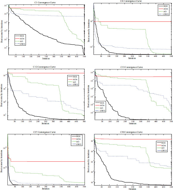
Figure 7. Comparative convergence curves for some of the CEC2017 benchmark functions
5. Conclusions
This paper has evaluated the performance of the gradient descent-based algorithms and swarm-based metaheuristic algorithms for the ANN training by using statistical metrics of MSE, MAE, and R2. Unlike other published studies that compare the performance of the metaheuristic algorithms and gradient descent-based algorithms amongst themselves, this paper takes a position from a wider perspective and performs the comparison between metaheuristic algorithms and gradient descent-based algorithms. Initially the stated algorithms have been compared in terms of MSE, MAE and R2 values. The metaheuristic algorithms have been found to be quite superior at this stage. Therefore, were further compared amongst themselves in terms of classification abilities and optimization of benchmark functions with different difficulties. The assessments have shown that the HGS algorithm can achieve more excellent results compared to the other swarm-based metaheuristic algorithms. The work presented in this paper will shed the light on future studies related to ANN training. Further performance improvements will make it possible to use various data sources and hybridized versions of the algorithms, combining both swarm-based metaheuristic and gradient descent-based algorithms. The latter can be investigated as a potential future work.
6. References
Abualigah, L., Yousri, D., Abd Elaziz, M., Ewees, A. A., Al-qaness, M. A., & Gandomi, A. H., 2021. Aquila Optimizer: A novel meta-heuristic optimization Algorithm. Computers & Industrial Engineering, 157, 107250. https://doi.org/10.1016/j.cie.2021.107250
Chong, H. Y., Yap, H. J., Tan, S. C., Yap, K. S., & Wong, S. Y., 2021. Advances of metaheuristic algorithms in training neural networks for industrial applications. Soft Computing, 25(16), 11209–11233. https://doi.org/10.1007/s00500-021-05886-z
Dragoi, E. N., & Dafinescu, V., 2021. Review of Metaheuristics Inspired from the Animal Kingdom. Mathematics, 9(18), 2335. https://doi.org/10.3390/math9182335
Devikanniga, D., Vetrivel, K., & Badrinath, N. (2019, November). Review of meta-heuristic optimization based artificial neural networks and its applications. Journal of Physics: Conference Series, 1362(1), 012074. https://doi.org/10.1088/1742-6596/1362/1/012074
Dogo E. M., Afolabi O. J., Nwulu N. I., Twala B., & Aigbavboa C. O., 2018. A Comparative Analysis of Gradient Descent-Based Optimization Algorithms on Convolutional Neural Networks. In 2018 International Conference on Computational Techniques, Electronics and Mechanical Systems (CTEMS) (pp. 92–99). https://doi.org/10.1109/CTEMS.2018.8769211
Eker, E., Kayri, M., Ekinci, S., & Izci, D., 2021. A new fusion of ASO with SA algorithm and its applications to MLP training and DC motor speed control. Arabian Journal for Science and Engineering, 46(4), 3889–3911. https://doi.org/10.1007/s13369-020-05228-5
Engy, E., Ali, E., & Sally, E.-G., 2018. An optimized artificial neural network approach based on sperm whale optimization algorithm for predicting fertility quality. Stud. Inform. Control., 27, 349–358. https://doi.org/10.24846/v27i3y201810
Eren, B., Yaqub, M., & Eyüpoğlu, V., 2016. Assessment of neural network training algorithms for the prediction of polymeric inclusion membranes efficiency. Sakarya Üniversitesi Fen Bilimleri Enstitüsü Dergisi, 20(3), 533–542. https://doi.org/10.16984/saufenbilder.14165
Fisher, R. A., 1936. The use of multiple measurements in taxonomic problems. Annals of eugenics, 7(2), 179–188. https://doi.org/10.1111/j.1469-1809.1936.tb02137.x
Ghaffari, A., Abdollahi, H., Khoshayand, M. R., Bozchalooi, I. S., Dadgar, A., & Rafiee-Tehrani, M.M., 2006. Performance comparison of neural network training algorithms in modeling of bimodal drug delivery. International journal of pharmaceutics, 327(1-2), 126–138. https://doi.org/10.1016/j.ijpharm.2006.07.056
Gardner, M. W., & Dorling, S. R., 1998. Artificial neural networks (the multilayer perceptron) —a review of applications in the atmospheric sciences. Atmospheric environment, 32(14-15), 2627–2636. https://doi.org/10.1016/S1352-2310(97)00447-0
Grippo, L., 2000. Convergent on-line algorithms for supervised learning in neural networks. IEEE transactions on neural networks, 11(6), 1284–1299. https://doi.org/10.1109/72.883426
Gupta, T. K., & Raza, K. (2019). Optimization of ANN architecture: a review on nature-inspired techniques. In Machine learning in bio-signal analysis and diagnostic imaging, 159–182. https://doi.org/10.1016/B978-0-12-816086-2.00007-2
Heidari, A. A., Faris, H., Aljarah, I., & Mirjalili, S., 2019. An efficient hybrid multilayer perceptron neural network with grasshopper optimization. Soft Computing, 23(17), 7941–7958. https://doi.org/10.1007/s00500-018-3424-2
Hornik, K., Stinchcombe, M., & White, H., 1989. Multilayer feedforward networks are universal approximators. Neural networks, 2(5), 359–366. https://doi.org/10.1016/0893-6080(89)90020-8
Haykin, S., 2005. Neural Networks: A Comprehensive Foundation, ninth edition Prentice-Hall, Upper Saddle River, NJ., 30–52.
Hecht-Nielsen, R., 1992. Theory of the backpropagation neural network. In Neural networks for perception (pp. 65–93). Academic Press. https://doi.org/10.1016/B978-0-12-741252-8.50010-8
Hashim, F. A., Hussain, K., Houssein, E. H., Mabrouk, M. S., & Al-Atabany, W., 2021. Archimedes optimization algorithm: a new metaheuristic algorithm for solving optimization problems. Applied Intelligence, 51(3), 1531–1551. https://doi.org/10.1007/s10489-020-01893-z
Jawad, J., Hawari, A. H., & Zaidi, S. J., 2021. Artificial neural network modeling of wastewater treatment and desalination using membrane processes: A review. Chemical Engineering Journal, 419, 129540. https://doi.org/10.1016/j.cej.2021.129540
Khan, A., Shah, R., Bukhari, J., Akhter, N., Attaullah; Idrees, M., & Ahmad, H., 2019. A Novel Chicken Swarm Neural Network Model for Crude Oil Price Prediction. In Advances on Computational Intelligence in Energy (pp. 39–58). Cham, Switzerland: Springer. https://doi.org/10.1007/978-3-319-69889-2_3
Khishe, M., & Mosavi, M., 2019. Classification of underwater acoustical dataset using neural network trained by Chimp Optimization Algorithm. Appl. Acoust., 157, 107005. https://doi.org/10.1016/j.apacoust.2019.107005
Kayri, M., 2015. An intelligent approach to educational data: performance comparison of the multilayer perceptron and the radial basis function artificial neural networks. Educational Sciences: Theory & Practice, 15(5).
Lv, Z., & Qiao, L., 2020. Deep belief network and linear perceptron based cognitive computing for collaborative robots. Applied Soft Computing, 92, 106300. https://doi.org/10.1016/j.asoc.2020.106300
Ly, H. B., Nguyen, M. H., & Pham, B. T., 2021. Metaheuristic optimization of Levenberg–Marquardt-based artificial neural network using particle swarm optimization for prediction of foamed concrete compressive strength. Neural Computing and Applications, 33(24), 17331–17351. https://doi.org/10.1007/s00521-021-06321-y
Shabani, M. O, & Mazahery, A., 2012. Prediction Performance of Various Numerical Model Training Algorithms in Solidification Process of A356 Matrix Composites. Indian Journal of Engineering and Materials Sciences, 19(2), 129–134.
Mirjalili, S., Mirjalili, S. M., & Lewis, A., 2014. Grey wolf optimizer. Advances in engineering software, 69, 46–61. https://doi.org/10.1016/j.advengsoft.2013.12.007
Mirjalili, S., 2015. How effective is the Grey Wolf optimizer in training multi-layer perceptrons. Applied Intelligence, 43(1), 150–161. https://doi.org/10.1007/s10489-014-0645-7
Mohamed, A. W., Hadi, A. A., & Mohamed, A. K., 2020. Gaining-sharing knowledge based algorithm for solving optimization problems: a novel nature-inspired algorithm. Int J Mach Learn Cybern, 11, 1501–1529. https://doi.org/10.1007/s13042-019-01053-x
Movassagh, A. A., Alzubi, J. A., Gheisari, M., Rahimi, M., Mohan, S., Abbasi, A. A., & Nabipour, N., 2021. Artificial neural networks training algorithm integrating invasive weed optimization with differential evolutionary model. Journal of Ambient Intelligence and Humanized Computing, 1–9. https://doi.org/10.1007/s12652-020-02623-6
Nguyen, H., & Bui, X. N., 2021. A novel hunger games search optimization-based artificial neural network for predicting ground vibration intensity induced by mine blasting. Natural Resources Research, 30(5), 3865–3880. https://doi.org/10.1007/s11053-021-09903-8
Paulin, F., & Santhakumaran, A., 2011. Classification of breast cancer by comparing back propagation training algorithms. International Journal on Computer Science and Engineering, 3(1), 327–332.
Ray, S., 2019, February. A quick review of machine learning algorithms. In 2019 International conference on machine learning, big data, cloud and parallel computing (COMITCon) (pp. 35–39). IEEE. https://doi.org/10.1109/COMITCon.2019.8862451
Sönmez Çakır, F., 2018. Yapay Sinir Ağları Matlab Kodları ve Matlab Toolbox Çözümleri, 1 Baskı, Nobel Kitabevi, Ankara.
Wang, W., Gelder, P. H. V., & Vrijling, J. K., 2007. Comparing Bayesian regularization and cross-validated early-stopping for streamflow forecasting with ANN models. IAHS Publications-Series of Proceedings and Reports, 311, 216–221.
Yang, Y., Chen, H., Heidari, A. A., & Gandomi, A. H., 2021. Hunger games search: Visions, conception, implementation, deep analysis, perspectives, and towards performance shifts. Expert Systems with Applications, 177, 114864. https://doi.org/10.1016/j.eswa.2021.114864