ADCAIJ: Advances in Distributed Computing and Artificial Intelligence Journal
Regular Issue, Vol. 13 (2024), e29191
eISSN: 2255-2863
DOI: https://doi.org/10.14201/adcaij.29191
CNN Based Automatic Speech Recognition: A Comparative Study
Hilal Ilgaza, Beyza Akkoyuna, Özlem Alpaya, and M. Ali Akcayola
a Computer Engineering Department, University of Gazi. Ankara, Turkey, 06570.
hilalilgaz06@gmail.com, beyzaakkoyun9@gmail.com, ozlemalpay@gazi.edu.tr, akcayol@gazi.edu.tr
ABSTRACT
Recently, one of the most common approaches used in speech recognition is deep learning. The most advanced results have been obtained with speech recognition systems created using convolutional neural network (CNN) and recurrent neural networks (RNN). Since CNNs can capture local features effectively, they are applied to tasks with relatively short-term dependencies, such as keyword detection or phoneme- level sequence recognition. This paper presents the development of a deep learning and speech command recognition system. The Google Speech Commands Dataset has been used for training. The dataset contained 65.000 one-second-long words of 30 short English words. That is, %80 of the dataset has been used in the training and %20 of the dataset has been used in the testing. The data set consists of one-second voice commands that have been converted into a spectrogram and used to train different artificial neural network (ANN) models. Various variants of CNN are used in deep learning applications. The performance of the proposed model has reached %94.60.
KEYWORDS
Deep learning; Artificial neural networks; Speech recognition
1. Introduction
Human-machine interfaces for smart machines such as smartphones, home robots, and autonomous vehicles should become commonplace in the future. Noise-tolerant speech recognition systems are very important to ensure effective human-machine interaction (Noda et al., 2015). Automatic speech recognition (ASR) is defined as a speech recognition or speech-to-text task. The first methods in the ASR problem included Gaussian mixture models (GMM), the dynamic time warping (DTW) algorithm, and hidden Markov models (HMM) (Rodríguez et al., 1997). It has been observed that the success in the ASR problem is greatly enhanced by the application of deep neural networks (DNNs) (Khanam et al., 2022). CNNs are generally used in the analysis of visual datasets. CNN’s have been used in speech recognition studies due to their success in reducing spectral changes and modeling spectral correlations of speech signals (Sainath et al., 2013). CNNs used in ASR systems take the spectrogram of speech signals represented as images as input and recognize speech using these features.
Most of the human-computer interfaces, such as Google Assistant, Microsoft Cortana, Amazon Alexa, Apple Siri, and others, rely on speech recognition. Besides, Google offers a voice search service and a completely hands-free experience called “Ok Google” on Android phones. There is a great deal of research being done by large companies in this area. Due to computational problems, speech recognition systems are based on neural network models operating in the cloud. These problems are converting speech to text and responding to conversation. Simple commands, such as “stop, go” can be processed locally and go through the same processing steps. The emergence of lightweight voice command systems has allowed for the development of many new engineering applications. For example, robots with voice control, critical and assistive devices can work without an internet environment. This feature is especially significant in the design of microcontrollers that support voice commands (Zhang et al., 2017; de Andrade et al., 2018).
2. Related Work
Andrade et al. have proposed a convolutional recurrent network using attention for speech command recognition (de Andrade., 2018). Attention approaches can improve natural language processing, image or video captioning, and speech recognition. The authors used the Google Speech Commands dataset in 2 different ways, using 35 words (V1) and 20 words (V2). The proposed model achieved an accuracy score of %94.1 in the V1 dataset, and an accuracy score of %94.5 in the V2 dataset.
Büyük has developed a Turkish speech recognition system for mobile devices (Büyük 2018). In this study, a new database has been created that includes recordings from different speakers and smartphones. The success of the developed model has been tested using three speech recognition applications, television control, SMS (short message service) and general text dictation. According to the experiments, %95 recognition has been realized in the grammar-based television control application. The accuracy in SMS and general text dictation applications is approximately %40 and %60 respectively.
Wang et al. have proposed an end-to-end generative text-to speech model that synthesizes speech directly from characters called Tacotron (Wang et al., 2017). Tacotron is a seq2seq model with attention. The model takes characters as input and produces spectrogram frames. The authors have performed voice synthesis with parameters similar to those in the Google Speech Commands dataset. It scored 3.82 out of 5 in US English. This proves that Tacotron performs well in terms of naturalness.
Noda et al. have presented the connectionist-hidden Markov model for noise-resistant audio-visual speech recognition (AVSR) (Noda et al., 2015). An automatic encoder has been used as a noise remover. CNN has been used to extract visual features from raw mouth area images. The hidden Markov model (HMM) is built with the data extracted in the first two stages. The word recognition rate of their system is 65.
Fantaye et al. have proposed models combining CNN and RNN to reduce speech recognition problems (Fantaye et al., 2020). These models are gated convolutional neural network model (GCNN), recurrent convolutional neural network model (RCNN), gated recurrent convolutional neural network model (GRCNN), highway recurrent convolutional neural network model (HRCNN), Res-RCNN and Res-RGCNN models. Experiments have been conducted on the Amharic, Chaha datasets, and on the limited language packages (10-h) of the benchmark datasets of the Intelligence Advanced Research Projects Activity (IARPA) Babel Program. The proposed neural network models achieved %0.1–42.79 relative performance improvements over six language collections.
Dridi et al. have developed two models that combine CNN, GRU-RNN and DNN called convolutional gated recurrent unit deep neural network (CGDNN) and convolutional long short-term memory deep neural network (CLDNN) (Dridi et al., 2020). Experiments have been conducted on the TIMIT data set. According to the experimental results, the CLDNN architecture provided an improvement of %0.99 compared to the training data set and 0.87 compared to the test data set, when compared to the DLSTM model. The CGDNN architecture provided a %0.22 improvement in the training dataset and %0.14 in the test dataset in recognition rates, compared to the CLDNN architecture.
McMahan and Rao have analyzed very deep convolutional networks to classify audio spectrograms (McMahan et al., 2018). The experiments were conducted on the UrbanSound8k and Google Speech Commands datasets. The deep convolutional networks that had been used were SB-CNN (Salamon and Bello, 2017), ResNet18, ResNet34, ResNet50, DenseNet121, DenseNet161 and DenseNet169. This study results are:
In studies with different sub models of CNN, accuracy scores without scaling are between %77 and %65.
It has been seen that DenseNet performs very well on audio spectrogram classification when compared to a baseline network and ResNet.
Keyword detection technology is a potential technique for providing a completely hands-free interface, which is more suitable for mobile devices than hand typing. It is an available technique for some emergencies such as driving a car. Speech command recognition systems are mostly run on smartphones or tablets. They must have low latency, have a very small memory footprint, and require only very small computation (O’Shaughnessy, 2008).
3. Material and Methods
3.1. Dataset
The Google Speech Commands Dataset (Warden 2018; Kolesau et al., 2021) is a voice dataset of spoken command words designed to help train and evaluate keyword determination systems. Its main aim is to make it easier to create and test small models that can recognize when a single word from a set of target words is spoken, with as few false positives as possible, which are caused by background noise or irrelevant speech. The dataset includes 65,000 one-second-long words of 30 short English words contributed by thousands of different people via the AIY website. There are also realistic background sound files that can be placed in the background of sounds to help training networks cope with noisy environments.
The way the dataset was prepared began with twenty basic command words, with most speakers saying them every five times. Keywords are “Yes”, “No”, “Up”, “Down”, “Left”, “Right”, “On”, “Off”, “Stop”, “Go”, “Zero”, “One”, It has been designated as “Two”, “Three”, “Five”, “Six”, “Seven”, “Eight” and “Nine”. There are also ten auxiliary words to help distinguish unrecognized words in this order. These are words that most speakers say only once: “Bed”, “Bird”, “Cat”, “Dog”, “Happy”, “House”, “Marvin”, “Sheila”, “Tree”, and “Wow” (Vygon et al., 2021).
During the data set preparation process, the possibilities of the existing computer hardware of the developers were taken into consideration, and the model setup process was carried out with 10 categories to be selected from the data set. Thus, the aim has been to make more improvement attempts using the time gained in the training phase. After the structure of the developed models was determined, a second evaluation process was carried out using all of the data (Andrade et al., 2018). The 10 categories used are as follows: ‘yes’, ‘no’, ‘up’, ‘down’, ‘left’, ‘right’, ‘on’, ‘off’, ‘stop’, ‘go’.
Audio recordings are saved as.wav files. The audio recordings had to be converted to digital data used for database creation. Thus, they were converted into the format used in the programming language. That is why Numpy was chosen. Numpy, short for Numerical Python is a Python software package that makes heavy use of linear algebra operations on a long list/vector/matrix of numbers (Numpy). The conversion to digital format was done in a file used for preprocessing before the database was created. A detailed analysis of the data was carried out. The original files must be in 16-bit little-endian PCM-encoded WAVE (Lee et al., 2017) format. The sampling rate (sampling frequency) was 16,000 by default (Warden, 2018).
The training and testing processes were carried out with different word groups consisting of 30 words in total and 10 words in divided form. In addition to these, “silence” and “unknown” categories were also used for training to ensure that the model would be successful in real-life applications. “Silence” includes all records that should be guessed silently, and “unknown” includes word records that should be guessed as unknown.
3.1.1. Collecting Data in wav Format
Unknown class: We have conducted the experiment by choosing 10 categories out of 30 categories, the remaining words are selected as an unknown class.
Background noise: Training is also required for recorded sounds with similar characteristics to create a noise-proof model. The files in the dataset were captured on various devices by users in many different environments, not in a studio. This situation adds realism to education. To best reflect the real situation within the paper, random environmental sounds are mixed into the training inputs.
Normal the sounds of interest would be paused in most cases. That is why it is important to know that there is no match sound. Since there is never complete silence in real environments, in the paper, we need to provide examples with quiet and irrelevant audio.
Silence: Normally, the sounds of interest would be paused. That is why it is important to know that there is no match sound. Since there is never complete silence in real environments, in the paper, we need to provide examples with quiet and irrelevant audio.
The wav file graph of the word “yes” is shown in Figure 1.
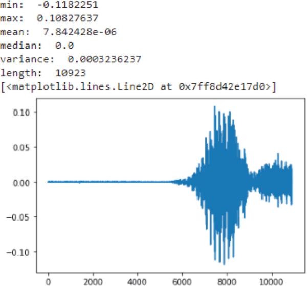
Figure 1. The wav file graph of the word “yes”
3.1.2. Transition from wav to Spectrogram
The Mel spectrogram is created from the amplitude data of the sound recordings. Following the literature review, the mel spectrogram was chosen because it best represents the acoustic properties. Therefore, Mel spectrograms have been frequently used in deep learning methods. The Mel scale spectrogram is calculated using the 85-band Mel scale, the length of the vector subjected to the fast Fourier transform (FFT) of 1024 and the jump size of 128 points (8s). Similar parameters have been used successfully for voice synthesis. We have noticed that these parameters preserve the visual aspect of the sound formatters in the spectrogram (this allows an expert to evaluate the sound (Sundberg et al., 2013).
A method has been prepared for the Mel spectrogram conversion process, and an array has been taken as the output of the method. The output array size is (122,85) for time and frequency. The Mel spectrogram scale of the word “yes” is shown in Figure 2.
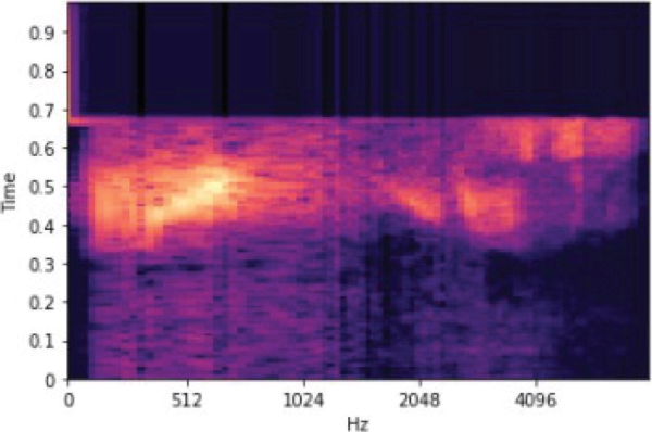
Figure 2. The Mel spectrogram scale of the word “yes”
The dataset used in the study includes 30 short words voiced by different people. Each word has a duration of one second and a total of 65,000 seconds long. First of all, the data preprocessing step is carried out. Audio frequency is one of the frequencies used for the transmission of speech. The frequencies of the sound recordings in this data set are 16000 hz. To work with sound files in Python, these frequencies should be 8000 hz. Therefore, the frequencies of the audio recordings in the dataset have been changed.
In an ASR problem, speech is converted into a mathematical representation known as a feature. Features provide ease of analysis and processing. The most common technique among all techniques used for feature extraction is; Mel-frequency cepstral coefficients (MFCC) due to its simplicity of calculation, low-dimensional coding, and success at the recognition stage. It is necessary to create a feature map according to the structure of the words used in the data set. Then, the data in this feature map forms the input data of the CNN.
In this study, MFCC features are arranged as one-dimensional. Here, one-dimensional feature maps are applied using the number of frames and filter banks. Figure 3 shows the process of obtaining the frequency from the raw sound signal. Figure 4 shows a convolutional neural network with full weight sharing applied along the frequency axis (Abdel-Hamid et al., 2013).
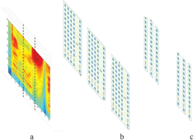
Figure 3. The process of obtaining frequency from the raw audio signal (a: Frame of raw audio signal b: 2D representation of this speech signal divided into frames, c: The normalized in the frequency domain)
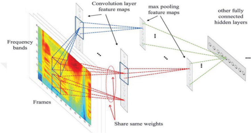
Figure 4. A convolutional neural network applied along the frequency axis
3.1.3. Training-Testing Data Split
For modeling and prediction, the data set should be divided into training and testing. The training data is randomly split into %80 of all the data, while the test data is randomly split into %20 Validation data is randomly split into %20 of the training data. X represents all the features of the data set, and Y represents the target variable. Class numbers are distributed differently for each word, starting from 1. While saving the data sets, the channel size for Keras is added, and at the same time, normalization is performed.
4. Experimental Design
Automatic speech recognition (ASR) is the process of converting audio signals into strings of words. Speech recognition allows one to follow and understand voice commands. ASR systems have been used in a variety of environments, including in applications that convert speech to text on smartphones, industrial fields, military (in fighter aircraft), recognition programs for disabled users, translation, and language learning, medical, office, and home.
Deep learning methods are frequently used to recognize words from speech signals. The paper has been mainly focused on a system that identifies the key features of the speech recognition system with deep learning and can convert audio to text files. In the created system, the conversion will continue if the user says certain commands.
Since the amount of data in the paper is very high, the data and the models to be used are decided according to the trial results. The CNN-based models are fitted to the data, and the results are obtained.
During the model development phase of the paper, experiments were carried out on the combination of CNN models, visual geometry group (VGG) models, and residual network (ResNet) models. The results were evaluated, and eliminations were made, and the most promising ones were focused on (Beckmann, Kegler et al. 2019, Poudel and Anuradha 2020, Kim, Chang et al. 2021, Vygon and Mikhaylovskiy 2021). In this section, these models are discussed. Two different training processes have been carried out as part of the project. The 10 words, namely, yes, no, up, down, left, right, on, off, stop and go, also include two different categories called silence and unknown. The second process included all 30 words and the silence category. Different training will be considered for these two trainings when presenting the results.
4.1. The CNN Model
CNN uses a standard neural network to solve classification problems (Cevik et al., 2020). For the study, the traditional model of CNN was tested with various variations. The best results from the standard model include four convolutional layers and two fully connected layers and a flatten layer. Each of the convolutional layers has a valid padding parameter. The activation function is the rectified linear unit (ReLU) and the stride number is 1. In research that seeks to tune CNNs for speech recognition tasks, only maxpooling on the frequency axis is added after the first convolutional layer. Therefore, we have also added max-pooling by the kernel size and stride value. We have applied dropout after all convolutional layers and fully connected layers. Softmax is applied in the output layer. The CNN model is shown in Figure 5.
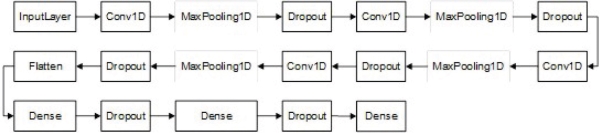
Figure 5. The CNN model
4.2. The VGGNet Model
The original VGG network (Simonyan et al., 2014) has five convolutional blocks. The first two of these each have a convolutional layer, and the last three each have two convolutional layers. Because this network uses 8 convolutional layers and 3 fully connected layers, it is often referred to as VGG-11 (Ruan, Zhao et al. 2022). The variant of the original VGG-11 that we designed in the paper consists of three blocks. The first two of these blocks have two convolutional layers. In the last block, there is 1 convolutional layer. In total, 5 convolutional layers and 3 connected layers are used. Regarding the activation functions, Softmax is used in the last layer and ReLU is used for the other fully connected layers. A value of 0.001 is accepted as the learning rate.
Results are obtained for Model 1 with 20 epochs, Batch-Size 100 and Model 2 with 50 epochs, Batch-Size 100 for 12 classes of training with 10 words and 2 additional classes. Model 3 with 20 epochs, 64 Batch-Size and model 4 with 50 epochs, Batch-Size of 64 for 31 class training. The VGGNet Model is shown in Figure 6.
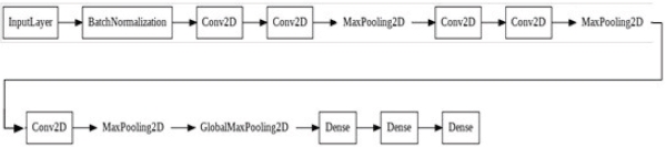
Figure 6. The VGGNet model
4.3. ResNet Model
A residual block 1, a residual block 2, and a model function are coded for the generated ResNet model (Wang et al., 2017b). The model has a convolutional layer and a fully connected layer. Residual block 1/0 has 1 convolutional layer. Residual block 2 has 3 convolutional layers. Softmax is used in the last layer as the activation function. A value of 0.001 is used for the learning rate. The ResNet Model is shown in Figure 7.
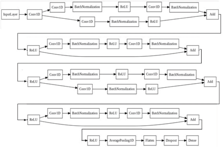
Figure 7. The ResNet model
5. Experimental Results
In this study, deep learning-based models have been developed for the speech recognition problem. The first problem that we have noticed in the testing process is that the samples belonging to the categories in the data content need to be in balanced numbers. Thus, the model training is also affected by this situation. In particular, the data redundancy in the unknown class affects this situation. Keras has a class-weight parameter in the fit function that imposes higher penalties for misclassifications in underrepresented classes. In addition, we have applied a weighting process to the classes. We also have used precision and recall scales as we have aimed to give a completely accurate assessment due to unbalanced data distribution.
As shown in Figure 8, VGGNet 2 and the ResNet model come to the fore. However, as mentioned before, test-training accuracy graph flow and test-training loss graph flow are also followed as evaluation criteria besides
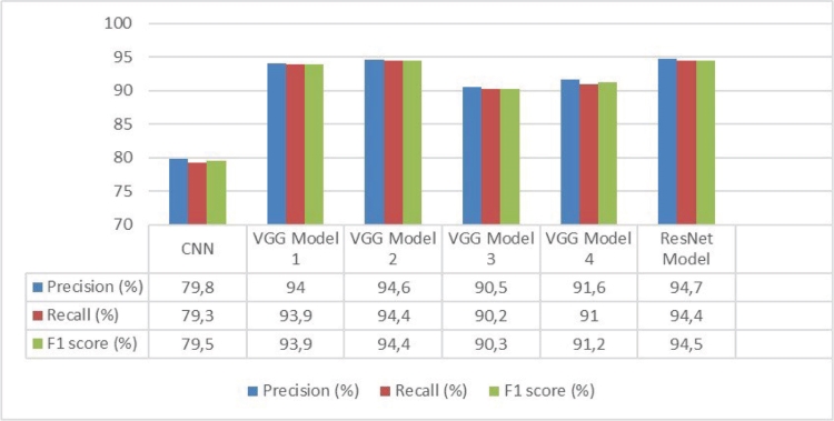
Figure 8. Comparison of models
precision and recall values. The ResNet model has high evaluation values, but it has been decided that it is a more unstable and therefore an unsafe graphic. In this direction, the outputs obtained for the VGG model 2, which gives the best results, are shown in Appendix A. A comparison of models is shown in Figure 8.
• CNN model features 64 batch, 100 epoch and 12 class
• VGG model 1 features 100 batch 20 epoch and 12 class
• VGG model 2 features 100 batch 50 epoch and 12 class
• VGG model 3 features 64 batch 20 epoch and 31 class
• VGG model 4 features 64 batch 50 epoch and 31 class
• ResNet model features 108 batch 50 epoch and 12 class
Each column represents a set of samples where each tag is predicted to be, so the first column shows all the clips predicted to be yes, and the second one shows all the clips predicted to be no. Each row represents clip with accurate and precise information tags. Therefore, the first column continues as all clips are predicted to be yes; in the second column, all the clips are predicted to be no.
The confusion matrix may be more available than the accuracy score as it also includes the errors made in the network. The first line contains all the clips with “yes.” It means that all of them are correctly labeled in this study. A false negative prediction has yet to be made for the word yes. This shows that it successfully distinguishes “yes” from other words. Upon examining the “up” column we can see non-zero values. The column shows all clips predicted to be “up”. Positive numbers outside the “up” cell are errors. This means that some spoken words are predicted as “up,” and there are a lot of false positives.
Table 1 is the summarized version of Appendix A. According to Appendix A, the diagonal elements of the matrix indicate the number of values for which the predicted class is equal to the actual class. The off-diagonal elements of the same matrix represent misclassified elements. The diagonal values of the confusion matrix are expected to be high because they show many correct predictions. In Table 1, for example, 11 data points with the ground truth label “down” are estimated as “no,” and 36 data points with the true label “down” are estimated as “go”. 24 data points with a ground truth label of “off” are estimated as “up”. Twenty-five data points with the ground truth label “happy” are estimated as “up”. Thirty data points with the ground truth label “three” are estimated to be “tree.” 11 data points with the ground truth label “tree” are estimated as “three”.
Table 1. Confusion matrix summarization with 31 classes for VGG model 4
Class Name |
TP |
FP |
FN |
Number of Samples |
Yes |
246 |
- |
- |
246 |
No |
244 |
11 = 11*Down |
- |
244 |
Up |
244 |
49 = 24*Off +25*Happy |
- |
244 |
Down |
200 |
- |
47 = 11*No + 36*Go |
247 |
Left |
232 |
- |
- |
232 |
Right |
246 |
- |
- |
246 |
On |
228 |
- |
- |
228 |
Off |
225 |
- |
- |
225 |
Stop |
222 |
- |
- |
222 |
Go |
237 |
- |
- |
237 |
Silence |
37 |
- |
- |
37 |
Dog |
157 |
- |
- |
157 |
Eight |
232 |
- |
- |
232 |
Bed |
186 |
- |
- |
186 |
Cat |
156 |
- |
- |
156 |
Bird |
152 |
- |
- |
152 |
Four |
257 |
- |
- |
257 |
Five |
216 |
- |
- |
216 |
Happy |
156 |
- |
- |
156 |
House |
163 |
- |
- |
163 |
Nine |
214 |
- |
- |
214 |
Marvin |
156 |
- |
- |
156 |
One |
211 |
- |
- |
211 |
Seven |
238 |
- |
- |
238 |
Six |
241 |
- |
- |
241 |
Sheila |
158 |
- |
- |
158 |
Two |
212 |
- |
- |
212 |
Tree |
152 |
30 = 30*Three |
11 = 11*Three |
166 |
Three |
224 |
11 = 11*Three |
30 = 30*Three |
224 |
Zero |
249 |
- |
- |
249 |
Wow |
161 |
- |
- |
161 |
6. Conclusions
In this study, deep learning-based speech recognition models have been proposed to create a keyword detection system that can detect predefined keywords. The model has the ability to detect sound recordings taken in different environments. The classes to be detected are compatible with the sound recordings, the pronunciations in the content of the sound recording files are correctly perceived, the sound recordings are not affected by the background sounds when they are converted to a spectrogram, the database is consistent, the established models obtained high success scores, as well as the graphics based on the epoch values. It tested whether the correct determination could be made in the sound recording files of the subjects with different sound waves.
The approximate performance of the developed model is as follows: The CNN model is %79, the VGG model 2 is %94, the VGG model 1 is %94, the ResNet model is %94, the VGG model 3 is %90, and the VGG model 4 is %91.
6.1. Conflict of interest
The authors have no conflict of interest in publishing this work.
6.2. Plagiarism
The work described has not been published previously (except in the form of an abstract or as part of a published lecture or academic thesis) and is not under consideration for publication elsewhere. No article with the same content will be submitted for publication elsewhere while it is under review by ADCAIJ, that its publication is approved by all authors and tacitly or explicitly by the responsible authorities where the work was carried out, and that, if accepted, it will not be published elsewhere in the same form, in English or in any other language, without the written consent of the copyright-holder.
6.3. Contributors
All authors have materially participated in the research and article preparation. All authors have approved the final article to be true.
7. References
Abdel-Hamid, O., Deng, L., & Yu, D. (2013). Exploring convolutional neural network structures and optimization techniques for speech recognition. Proc. Interspeech, 2013, 3366-3370. https://doi.org/10.21437/Interspeech.2013-744
Beckmann, P., Kegler, M., Saltini, H., & Cernak, M. (2019). Speech-vgg: A deep feature extractor for speech processing. arXiv preprint arXiv:1910.09909.
Büyük, O. (2018). Mobil araçlarda Türkçe konus¸ma tanıma için yeni bir veri tabanı ve bu veri tabanı ile elde edilen ilk konus¸ma tanıma sonuçları. Pamukkale Üniversitesi Mühendislik Bilimleri Dergisi, 24(2), 180-184.
Cevik, F., & Kilimci, Z. H. (2020). Derin öğrenme yöntemleri ve kelime yerleştirme modelleri kullanılarak Parkinson hastalığının duygu analiziyle değerlendirilmesi. Pamukkale Üniversitesi Mühendislik Bilimleri Dergisi, 27(2), 151-161.
De Andrade, D. C., Leo, S., Viana, M. L. D. S., & Bernkopf, C. (2018). A neural attention model for speech command recognition. arXiv preprint arXiv:1808.08929.
Dridi, H., & Ouni, K. (2020). Towards robust combined deep architecture for speech recognition: Experiments on TIMIT. International Journal of Advanced Computer Science and Applications (IJACSA), 11(4), 525-534. https://doi.org/10.14569/IJACSA.2020.0110469
Fantaye, T. G., Yu, J., & Hailu, T. T. (2020). Advanced convolutional neural network-based hybrid acoustic models for low-resource speech recognition. Computers, 9(2), 36. https://doi.org/10.3390/computers9020036
Khanam, F., Munmun, F. A., Ritu, N. A., Saha, A. K., & Firoz, M. (2022). Text to Speech Synthesis: A Systematic Review, Deep Learning Based Architecture and Future Research Direction. Journal of Advances in Information Technology, 13(5). https://doi.org/10.12720/jait.13.5.398-412
Kim, B., Chang, S., Lee, J., & Sung, D. (2021). Broadcasted residual learning for efficient keyword spotting. arXiv preprint arXiv:2106.04140. https://doi.org/10.21437/Interspeech.2021-383
Kolesau, A., & Šešok, D. (2021). Voice Activation for Low-Resource Languages. Applied Sciences, 11(14), 6298. https://doi.org/10.3390/app11146298
Lee, J., Kim, T., Park, J., & Nam, J. (2017). Raw waveform-based audio classification using sample-level CNN architectures. arXiv preprint arXiv:1712.00866.
McMahan, B., & Rao, D. (2018, April). Listening to the world improves speech command recognition. In Proceedings of the AAAI Conference on Artificial Intelligence, 32(1). https://doi.org/10.1609/aaai.v32i1.11284
Noda, K., Yamaguchi, Y., Nakadai, K., Okuno, H. G., & Ogata, T. (2015). Audio-visual speech recognition using deep learning. Applied intelligence, 42, 722-737. https://doi.org/10.1007/s10489-014-0629-7
Numpy. (n.d.) What is NumPy . https://numpy.org/doc/stable/user/whatisnumpy.html
O’Shaughnessy, D. (2008). Automatic speech recognition: History, methods and challenges. Pattern Recognition, 41(10), 2965-2979. https://doi.org/10.1016/j.patcog.2008.05.008
Poudel, S., & Anuradha, R. (2020). Speech command recognition using artificial neural networks. JOIV: International Journal on Informatics Visualization, 4(2), 73-75. https://doi.org/10.30630/joiv.4.2.358
Rodríguez, E., Ruíz, B., García-Crespo, Á., & García, F. (1997). Speech/speaker recognition using a HMM/GMM hybrid model. In Audio-and Video-based Biometric Person Authentication: First International Conference, AVBPA’97 Crans-Montana, Switzerland, March 12-14, 1997 Proceedings 1 (pp. 227-234). Springer Berlin Heidelberg. https://doi.org/10.1007/BFb0016000
Ruan, K., Zhao, S., Jiang, X., Li, Y., Fei, J., Ou, D.,... & Xia, J. (2022). A 3D fluorescence classification and component prediction method based on VGG convolutional neural network and PARAFAC analysis method. Applied Sciences, 12(10), 4886. https://doi.org/10.3390/app12104886
Sainath, T. N., Kingsbury, B., Mohamed, A. R., Dahl, G. E., Saon, G., Soltau, H.,... & Ramabhadran, B. (2013, December). Improvements to deep convolutional neural networks for LVCSR. In 2013 IEEE workshop on automatic speech recognition and understanding (pp. 315-320). IEEE. https://doi.org/10.1109/ASRU.2013.6707749
Salamon, J., & Bello, J. P. (2017). Deep convolutional neural networks and data augmentation for environmental sound classification. IEEE Signal processing letters, 24(3), 279-283. https://doi.org/10.1109/LSP.2017.2657381
Simonyan, K., & Zisserman, A. (2014). Very deep convolutional networks for large-scale image recognition. arXiv preprint arXiv:1409.1556.
Sundberg, J., Lã, F. M., & Gill, B. P. (2013). Formant tuning strategies in professional male opera singers. Journal of Voice, 27(3), 278-288. https://doi.org/10.1016/j.jvoice.2012.12.002
Vygon, R., & Mikhaylovskiy, N. (2021). Learning efficient representations for keyword spotting with triplet loss. In Speech and Computer: 23rd International Conference, SPECOM 2021, St. Petersburg, Russia, September 27-30, 2021, Proceedings 23 (pp. 773-785). Springer International Publishing. https://doi.org/10.1007/978-3-030-87802-3_69
Wang, Y., Deng, X., Pu, S., & Huang, Z. (2017a). Residual convolutional CTC networks for automatic speech recognition. arXiv preprint arXiv:1702.
Wang, Y., Skerry-Ryan, R. J., Stanton, D., Wu, Y., Weiss, R. J., Jaitly, N.,... & Saurous, R. A. (2017b). Tacotron: Towards end-to-end speech synthesis. arXiv preprint arXiv:1703.10135.
Warden, P. (2018). Speech commands: A dataset for limited-vocabulary speech recognition. arXiv preprint arXiv:1804.03209.
Vygon, R., & Mikhaylovskiy, N. (2021). Learning efficient representations for keyword spotting with triplet loss. In Speech and Computer: 23rd International Conference, SPECOM 2021, St. Petersburg, Russia, September 27-30, 2021, Proceedings 23 (pp. 773-785). Springer International Publishing. https://doi.org/10.1007/978-3-030-87802-3_69
Zhang, Y., Suda, N., Lai, L., & Chandra, V. (2017). Hello edge: Keyword spotting on microcontrollers. arXiv preprint arXiv:1711.07128.
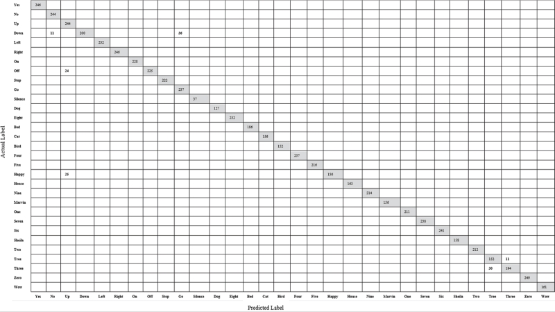
Appendix: A. Model confusion matrix output with 31 classes for VGG model 4