ADCAIJ: Advances in Distributed Computing and Artificial Intelligence Journal
Regular Issue, Vol. 12 N. 1 (2023), e29120
eISSN: 2255-2863
DOI: https://doi.org/10.14201/adcaij.29120
Object Detection and Regression Based Visible Spectrophotometric Analysis: A Demonstration Using Methylene Blue Solution
Ersin Aytaç
Department of Environmental Engineering, Zonguldak Bülent Ecevit University, 67100, Zonguldak, TÜRKÝYE
ABSTRACT
This study investigates the estimation of the concentration of methylene blue solutions to understand if visible spectrophotometry could be performed using a smartphone and machine learning. The presented procedure consists of taking photos, detecting test tubes and sampling region of interest (ROI) with YOLOv5, finding the hue, saturation, value (HSV) code of the dominant color in the ROI, and regression. 257 photos were taken for the procedure. The YOLOv5 object detection architecture was trained on 928 images and the highest mAP@05 values were detected as 0.915 in 300 epochs. For automatic ROI sampling, the YOLOv5 detect.py file was edited. The trained YOLOv5 detected 254 out of 257 test tubes and extracted ROIs. The HSV code of the dominant color in the exported ROI images was determined and stored in a csv file together with the concentration values. Subsequently, 25 different regression algorithms were applied to the generated data set. The extra trees regressor was the most generalizing model with 99.5% training and 99.4% validation R2 values. A hyperparameter tuning process was performed on the extra trees regressor and a mixed model was created using the best 3 regression algorithms to improve the R2 value. Finally, all three models were tested on unseen data and the lowest MSE value was found in the untuned extra trees regressor and blended model with values of 0.10564 and 0.16586, respectively. These results prove that visible spectrophotometric analysis can be performed using the presented procedure and that a mobile application can be developed for this purpose.
KEYWORD
Concentration Measurement; Machine learning; Image Regression; Object Detection; Visible Spectrophotometry; YOLOv5
1. Introduction
The recent decade witnessed the exciting success of machine learning in many areas, from bioinformatics to transportation (Aytaç, 2020; Arpaia et al., 2021). Breakthroughs in computer science theory, algorithmic analysis, and computational power have created methods for extracting useful knowledge from big data (Milojevic-Dupont and Creutzig, 2021). As a result, a new scientific field named machine learning (ML) has emerged. Since Arthur Samuel came up with the concept of "machine learning" in 1959, the rising popularity of this concept is making judgments in many areas (Aytaç and Khayet, 2023a). Machine learning uses unique approaches that allow computers to design interactions, forecast future events accurately and reveal complex underlying dynamics (Duysak and Yigit, 2020; Dogan and Birant, 2021; Aytaç, 2021a; Aytaç, 2022a; Khayet, 2022). These approaches can either be supervised, unsupervised, or reinforced. Supervised learning methods, that include classification or regression, may train a classifier to predict new data using known inputs and outputs. Unsupervised learning methods such as clustering, dimensionality reduction, anomaly detection and density estimation can uncover hidden patterns in the provided data. Reinforcement learning algorithms may learn from prior experiences and determine the best actions to take in an unknown environment to accomplish the optimal state transition for achieving the objective (Aytaç and Khayet, 2023b; Aytaç et al. 2023c; Aytaç et al. 2023d). Some of the research using these three branches of ML include robust fall detection in video surveillance (Lian et al., 2023), fire recognition (Sun et al., 2022), diagnosing Alzheimer’s disease using brain magnetic resonance imaging scans (Liu et al., 2023), temporal dynamic vehicle-to-vehicle interactions (Guha et al., 2022), to control chaos synchronization between two identical chaotic systems (Cheng et al., 2023), scheduling parallel processors with identical speedup functions (Ziaei and Ranjbar, 2023), controller for dynamic positioning of an unmanned surface vehicle (Yuan and Rui, 2023). Machine learning approaches still require development to be able to create high-quality predictive models, especially in situations where causal relationships between variables are difficult to fully resolve (Aytaç, 2021b, Aytaç 2022b).
Object detection, which is currently one of the most important areas of computer vision, aims to detect objects in real images from a wide number of specified categories (Liu et al., 2021). The object detection model usually returns proposed locations, class labels, and confidence scores for objects of a particular class (Solovyev et al., 2021). This type of application is very critical in many fields, including face recognition, autonomous driving, and medical imaging studies (Shuang et al., 2021). Supervised learning is the concept of learning from data using a labeled training dataset (Pereda and Estrada, 2019, Aytaç and Khayet, 2023d). This approach aims to create a relationship between the inputs and the outputs. The goal of supervised learning is to forecast the outcomes of a sequence of inputs that had not been used during learning (Osarogiagbon et al. 2021). Regression is an essential branch of supervised learning. Regression analysis is structured to approximate the relationship between a dependent variable and a series of independent variables by using a statistical approach (de Carvalho et al., 2020). Machine learning has taken the lead in regression problems over the last decade because traditional regression algorithms have difficulty handling discrete or tuned data (especially in multivariate regression) (Chen and Miao, 2020). Regression analyses is now very popular for handling prediction tasks because it is interpretable and simple (Chung et al, 2020).
Spectrophotometric analysis (spectrophotometry) has various applications and is an effective technique for routine analysis since it is affordable, simple to run, and usable in all laboratories (Ebraheem et al., 2011; Danchana et al., 2019; Ayman et al., 2020). Spectrophotometry is based on the measurement of the absorption of light by the sample under investigation in the visible and near-ultraviolet range (García-González et al., 2020). These analyses rely on the measurement of the absorbance of solutions and are comparative practices based on calibration curves and are practical tools in chemical analysis (Zayed et al., 2017; Marczenko and Balcerzak, 2000). Spectrophotometric processes take an important role in many areas such as coronal tooth discoloration (Chen, et al., 2020), dental bleaching (Claudino et al., 2021), drug (Arabzadeh et al., 2019), hematite/magnetite nanocomposites (Zayed et al., 2017), eye preparations, vial and drops (Ragab et al., 2018), dye removal (Huong et al., 2020; Pradhan et al., 2020) and metal content (Kukielski et al., 2019) analysis. The devices used in the spectrophotometric analysis are called spectrophotometers. Spectrophotometers can detect minor color variations that human eyes cannot notice (Perroni et al., 2017). The most used spectrophotometers are ultraviolet (UV), ultraviolet-visible (UV-VIS), fluorescence, solid-phase, Fourier-transform infrared spectroscopy (FTIR), Raman, and surface-enhanced Raman spectroscopy (SERS) (Dumancas et al., 2017). Among them, UV-VIS spectrophotometer is one of the most common techniques used to determine the concentration of dyes (color) in solutions, as it can measure the intensity of light in the visible spectrum as well as the ultraviolet spectrum (Bunnag et al., 2020; García-González et al., 2020). Visible spectroscopy is a precise and accurate approach in measuring the colors or color mixtures that our eyes detect (Eyring, 2003). The visible spectrum of light is the part of the electromagnetic spectrum that the human eye can see (as colors) with the lower limit between 360 and 400nm and the upper limit between 760 and 830nm (Sliney, 2016). Visible spectroscopy is a common measurement technique in science and engineering. Ariaeenejad et al., (2021) and Soni et al., (2020) used UV-VIS for methylene blue measurement, Priya et al. (2020) used for eosin yellow measurement, Wang et al. (2020) used for crystal violet measurement, and Pal et al., (2021) used for Congo red measurement. Due to the lack of financial mechanisms and service institutions, many laboratories in developing and less developed countries find it difficult to use spectrophotometer (Kandi and Charles, 2019). The use of mobile phones can be an alternative to overcome this problem. The use of smartphones has increased significantly across the world (Hao et al., 2020). Mobile phones and artificial intelligence are already in use in many areas, such as the detection and management of atrial fibrillation (Turchioe et al., 2020), automatic detection of children on mobile devices (Nguyen et al., 2019), emotion recognition (Zualkernan et al., 2017) and facial recognition (Azimi and Pacut, 2020). There are also studies on mobile phone colorimetry in the literature. However, in the conducted studies, the measurement requires a fixed distance, constant light intensity and additional equipment such as a closed chamber (Sumriddetchkajorn et al., 2013; Masawat et al., 2015; Afshari and Dinari, 2020).
This study proposes a framework to demonstrate that concentration measurements in the visible spectrum (colored samples) can be made quickly using a smartphone, without the need for traditional measuring devices. Furthermore, this work provides an alternative method for concentration measurements to be made in laboratories or schools that cannot afford a spectrophotometer/colorimeter device. Three significant points distinguish the presented study from others in the literature. 1 – The proposed method does not require a fixed light source or closed chamber for concentration measurement. 2 – This method can be used for photos taken from different distances, so there is no need for a fixed distance for the measurement. 3 – The presented study uses different regression algorithms and selects the model with the lowest loss function to obtain more accurate results. The procedure consists of four steps. In the first step, the photos of the solutions were taken remotely using a smartphone. Second, the test tubes in the photos were identified and automatically sampled from the region of interest (ROI) using the You-Only-Look-Once (YOLO)-v5 object detection algorithm. In the third step, the hue-saturation-value (HSV) code of the most common color in the samples was extracted and saved in the csv file along with the concentration value. Finally, the extracted data were processed with various regression algorithms and concentration estimates were made. The main sections of the study are illustrated in Figure 1.
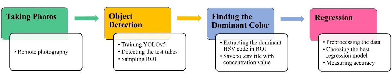
Figure 1. The flow chart of the process
2. Methodology
2.1. Taking Photos
Methylene blue solutions with concentrations ranging from 0 to 250 mg/L used in the study. The photos were taken remotely with a smartphone using a remote-control application in different lighting conditions on a fixed white background. The purpose of taking the photos remotely was to avoid measuring incorrect brightness values by blocking the light. 257 images were taken from distances of 20, 30 and 40 cm. The setup and some of the collected photos are shown in Figures 2 and 3, respectively.
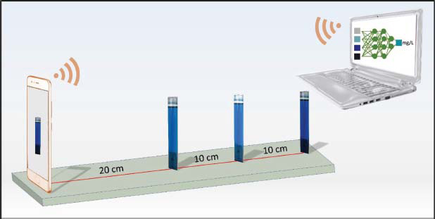
Figure 2. The setup used for photography
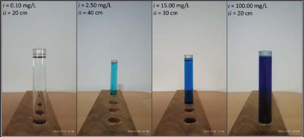
Figure 3. Some examples of the photos taken for the procedure (i = concentration, ii = distance to camera)
2.2. Object Detection
The fifth version of the YOLO object detection algorithm was used to determine the location of test tubes on images and to automatically sample the ROI. Glenn Jocher of Ultralytics LLC5 first released YOLOv5 in May 2020 (Jocher et al., 2021). YOLO is a coherent algorithm for real-time detection that reformulates the detection function as a single regression problem (Yap et al., 2020). The YOLOv5 module uses a single neural network architecture to find the object in the image with class probability and bounding boxes. The architecture was first implemented as part of a network known as Darknet (Vishwakarma and Vennelakanti, 2020). Publicly available test tube images were used to train this algorithm. For image augmentation, the dataset was increased to 928 using the imgaug library in Python (Jung, 2018) and split 80/20 as train/test data. Some examples of the augmented images used to train YOLOv5 are shown in Figure 4.
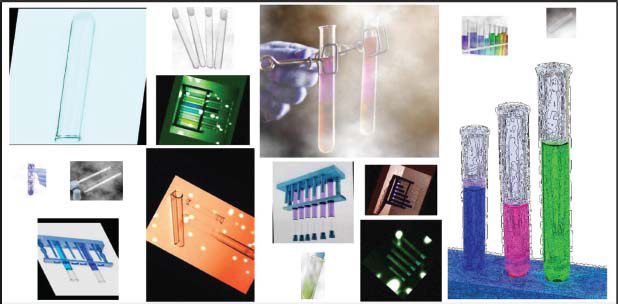
Figure 4. Some of the augmented images used in the object detection training process
One of the important points of the study is to take samples from the ROI of the detected test tubes. This was done by editing the detect.py file, which is used for the object detection step of the YOLOv5 algorithm. The following simple code was implemented in the detect.py file after line 114. This additional line extracted a 100x100 pixel sample from the ROI of the image. The center of the ROI was the center of the bounding box on the x-axis and 30 % of its height on the y-axis. The pseudo-code for the ROI extraction is given in Table 1.
Table 1. Pseudocode of ROI extraction (added to detect.py file after Line 114).
1: det ← detection |
2: im0 ← image file in detection |
3: img_ ← format changed image file in detection |
4: save_img ← if called save the cropped image |
5: xyxy ← an array containing the coordinates of the four corners of the bounding box |
6: xc ← center of the x coordinate of the bounding box |
7: yc ← center of the y coordinate of the bounding box |
8: h ← height of the bounding box |
9: h2 ← 20 % of the height of the bounding box |
10: if save_img |
11: for every det: |
12: find xc by adding xyxy[0] and xyxy[2] and divide by two |
13: find yc by adding xyxy[1] and xyxy[3] and divide by two |
14: find h by subtracting xyxy[1] from xyxy[2] |
15: find h2 by multiplying h by 0.3 |
16: change format of im0 to unsigned integer |
17: crop img_ from the desired coordinates (in this study yc-h2:yc-h2+100, xc-50:xc+50) |
18: save crop to the desired path with the name of im0 |
2.3. Finding the Dominant Color
The HSV color space highlights the visual variants of hue (H), saturation (S), and value (sometimes referred to as intensity or brightness) (V) of an image pixel (Bora et al., 2015). The HSV color in a three-dimensional space is a hexagon and the central vertical axis of this hexagonal structure represents the brightness (V). The apparent reflectance of a surface or the relative luminous reflectance of a colored surface patch is referred to as V. When an image is captured with a digital camera, V in the HSV code of the pixel is also a marker of the intensity of ambient light around the camera. The chromatic property that represents a pure color in the HSV space is hue and hue is represented as an angle between 0 degrees and 360 degrees. The saturation variable is the radial distance from the central axis and is described as the vitality of the color (Sural et al., 2002; Garcia-Lamont et al., 2018). The HSV color space has some important features, such as brightness, which are decoupled from the hue data. The H and S features mimic the human perception of color, so these HSV color space components become a valuable approach for developing image processing algorithms, and also this color space is useful for matching colors or suitable for determining whether one color is similar to another color (Cardani, 2001; Garcia-Lamont et al., 2018). The HSV color space attempts to accurately explain visual color associations precisely and the color segmentation of an image is relatively easy in the color space. The Python OpenCV library was used to determine the HSV code of the most common color in the samples. The concentration values of the samples, together with the HSV codes, were then recorded in a csv file, providing the necessary dataset for the regression process. The pseudo-code for extracting the dominant HSV code and saving it to a csv file with the concentration value, is given in Table 2.
Table 2. Pseudo-code of HSV extraction on ROI and saving to a csv file with concentration value.
1: path ← the path of images |
2: namelist ← a list of the names of the images (names are the concentrations) |
3 HSV_codes ← a list to store HSV codes |
4: dominant_RGB← most repeating RGB code in the image |
5: array_RGB← array form of RGB code |
6: nrm_array_RGB ← normalized RGB values (by dividing 255) |
7: dominant_HSV ← convert normalized dominant RGB code to HSV |
8: for every image in path: |
9: find dominant_RGB |
10: convert dominant_RGB to array_RGB |
11: normalize array_RGB |
12: covert array_RGB to dominant_HSV |
13: add dominant_HSV to HSV_codes list |
14: save HSV_codes to csv |
15: add namelist to saved csv |
The illustration of the test tube detection, sampling of ROI, and creating the csv file for the regression process stage can be seen in Figure 5.

Figure 5. Illustration of object detection, sampling and creating csv file steps (i = concentration, ii = distance to camera)
2.4. Regression
The regression process was performed using the Python PyCaret library on Google Colaboratory. PyCaret is a low-code, open-source Python environment for machine learning applications. PyCaret uses 25 different algorithms for regression and sorts the results according to the desired accuracy measure (Ali, 2020). In the process, the specifications of the computer assigned by Google Colaboratory are as follows: Tesla K80 graphical processing unit (GPU) (2496 CUDA cores, 12GB GDDR5 VRAM), 2.3 GHz Intel(R) Xeon(R) central processing unit (CPU), 13 GB random access memory (RAM), 33 GB of storage. In real-world applications of spectrophotometry, researchers first prepare a suitable calibration curve with a high R2 value (> 99 %) using standard solutions and then measure the concentrations of unknown samples using this calibration curve. In this study, however, the images were taken as a whole; not separated into standard solutions and unknown samples. First, all solutions were photographed and then the data set was divided into training/validation data and unknown samples using 500 random state values to generate an acceptable calibration curve (to create a generalized model). Random state values were selected using the criteria of training R2 > 99.4% and training/validation R2 difference < 0.1%.
The regression pipeline in the study is as follows. The first step in the regression process was to leave 10 % of the photos as unseen data (unknown samples) for the concentration measurement. The initial setup of the data was then performed. The data set was split into 80/20% training/validation data (to see if the model was overfitting or underfitting). The next step was to apply different regression algorithms with tenfold cross-validation to the training data and find the best model with the desired evaluation metric. The selection of the appropriate regressor was done depending on the target loss function (R2), as the evaluation of the accuracy of the calibration curve in UV-VIS spectroscopy is done on this value (Aragaw and Angerasa, 2020; Mijinyawa et al., 2020; Mokhtari et al., 2020). The training data can be considered as the standard solution used for the calibration curve.
Three different regression approaches were applied to the data set. First, a generalized model was determined, and the regression process was run. Second, the generalized model was hyper-parameterized to see if the scoring metrics could be improved and the regression process was run again. Third, the top 3 regressors were mixed (VotingRegressor) to evolve the model. A VotingRegressor could combine individual regressors to overcome the weaknesses of different regression algorithms and achieve more accurate prediction results (Pedregosa et al., 2011).
3. Results and Discussion
3.1. Object Detection
The object detection process started with the training of the YOLOv5 algorithm on 928 augmented images. The evaluation metrics of the training process of YOLOv5 for test tube detection after 300 epochs can be seen in Figure 6.

Figure 6. Training results of YOLOv5
As can be seen in Figure 6, the precision, mean precision, and recall values indicate that the training process was at a sufficient level. The mAP@05 value was around 0.880 after 30 epochs and the best mAP@05 value reached 0.915. A recognition process was then performed on the recorded images (conf. = 0.50, iou = 0.50). The trained YOLOv5 model detected 254 test tubes on 257 images and automatically sampled the ROIs. Figure 7 shows some of the detected test tubes (with bounding boxes and confidence values) and sampled ROIs.

Figure 7. Examples of the object detection algorithm results and sampled ROIs (i = concentration, ii = distance to the camera, iii = sampled ROI)
3.2. Finding the Dominant Color
The HSV code of the most repetitive color in the ROI was extracted using the Python OpenCV library. The extracted HSV codes and the concentration values of the samples were stored in a csv file. Thus, an image was transformed into an array form containing 3 independent variables (HSV codes) and 1 dependent variable (concentration).
3.3. Regression
To generate an acceptable calibration curve and to generalize the model, 500 (0-499) random state values were investigated. The regression pipeline was as follows.
1. Split data set as training/validation data and unseen data by 90/10 % (229 and 25 data instances respectively);
2. Split training and validation data by 80/20 % (183 and 46 data instances, respectively);
3. Transform training and validation data with Yeo–Johnson power transformation;
4. Run 25 different regression algorithms on the data set.
The results of the regression process (top 10 regressors) obtained for the random state value matching the desired criteria (training R2 > 99.4 % and training-validation R2 difference < 0.1 %) with 10-fold cross validation are given in Table 3. The extra trees regressor (ETR) seemed to be the most appropriate model for our data set for random state = 449 and default hyperparameter model seemed to be the most appropriate one for the regression process and the rest of the study focused on this model.
Table 3. Results of top 10 regressors
Random State Value |
Regressor |
Training Data |
Validation Data |
|||||||||||
MAE |
MSE |
RMSE |
R2 |
RMSLE |
MAPE |
Training Time (Sec) |
MAE |
MSE |
RMSE |
R2 |
RMSLE |
MAPE |
||
449 |
Extra Trees Regressor |
1.25298 |
8.14753 |
2.57213 |
0.99455 |
0.11696 |
0.16968 |
0.605 |
1.7272 |
31.2702 |
5.59198 |
0.99365 |
0.07407 |
0.08757 |
Decision Tree Regressor |
0.92914 |
7.22099 |
2.40193 |
0.99250 |
0.14787 |
0.14958 |
0.007 |
1.27337 |
16.57746 |
4.07154 |
0.99663 |
0.15158 |
0.20682 |
|
Gradient Boosting Regressor |
1.56181 |
22.83821 |
3.31745 |
0.98885 |
0.13134 |
0.25269 |
0.045 |
1.71425 |
21.53229 |
4.64029 |
0.99563 |
0.13614 |
0.25947 |
|
Random Forest Regressor |
1.57843 |
13.98472 |
3.23288 |
0.98851 |
0.22159 |
0.68882 |
0.619 |
1.49449 |
13.63501 |
3.69256 |
0.99723 |
0.10269 |
0.11856 |
|
K Neighbors Regressor |
2.08282 |
29.58803 |
4.78405 |
0.98482 |
0.11891 |
0.21975 |
0.014 |
2.24217 |
81.739708 |
9.041 |
0.98341 |
0.12046 |
0.20254 |
|
AdaBoost Regressor |
2.89411 |
16.42652 |
3.90242 |
0.97419 |
0.56640 |
3.70735 |
0.049 |
3.18794 |
20.84402 |
4.56553 |
0.99577 |
0.71798 |
5.25636 |
|
CatBoost Regressor |
2.43114 |
85.56710 |
6.29542 |
0.96816 |
0.17426 |
0.59687 |
0.458 |
1.99895 |
22.56725 |
4.7505 |
0.99542 |
0.12249 |
0.35886 |
|
Light Gradient Boosting Machine |
7.40420 |
321.28670 |
15.06040 |
0.81308 |
0.87671 |
7.88885 |
0.021 |
7.23332 |
271.38206 |
16.47368 |
0.94491 |
0.78033 |
7.09957 |
|
Multi Layer Perceptron Regressor |
11.52840 |
788.25319 |
24.28148 |
0.56309 |
1.07235 |
12.81037 |
0.374 |
17.91722 |
2008.4313 |
44.81553 |
0.59229 |
0.92969 |
7.27973 |
|
Huber Regressor |
13.17741 |
1189.5149 |
29.03141 |
0.51857 |
1.12809 |
13.99388 |
0.009 |
23.32686 |
3356.1778 |
57.93253 |
0.3187 |
1.06128 |
7.5072 |
|
These training and validation R2 values of ETR showed that both a suitable calibration curve was created, and the model did not overfit/underfit. After the selection of the generalized model, a hyperparameter tuning process was carried out to enhance the R2 value with 3000 iterations and 10-fold cross-validation. The results of the hyperparameter tuning process can be seen in Table 4.
Table 4. Hyperparameter tuning results for ETR
Training Data |
Validation Data |
|||||||||||
MAE |
MSE |
RMSE |
R2 |
RMSLE |
MAPE |
Training Time (Sec) |
MAE |
MSE |
RMSE |
R2 |
RMSLE |
MAPE |
1.62446 |
10.04622 |
2.83817 |
0.99249 |
0.18867 |
0.66047 |
>12000 |
2.83965 |
78.5524 |
8.86298 |
0.98405 |
0.19296 |
0.64616 |
Unfortunately, after 3000 iterations with more than 3 hours of grid search, hyperparameter tuning did not achieve the desired improvement. Considering the time taken, it would be unreasonable to use tuning as it goes against the idea of the rapid concentration measurement purpose of the method. In addition, a mixed model called VotingRegressor was introduced to check if better evaluation metrics could be achieved using the top 3 regressors (extra trees regressor, decision tree regressor and gradient boosting regressor). The training and validation results of the blended regressor with default hyperparameters are shown in Table 5.
Table 5. VotingRegressor results (regressors = extra trees regressor, decision tree regressor, and gradient boosting regressor)
Training Data |
Validation Data |
|||||||||||
MAE |
MSE |
RMSE |
R2 |
RMSLE |
MAPE |
Training Time (Sec) |
MAE |
MSE |
RMSE |
R2 |
RMSLE |
MAPE |
1.20855 |
7.92201 |
2.37064 |
0.99431 |
0.11093 |
0.15918 |
<12000 |
1.23224 |
9.49436 |
3.08129 |
0.99807 |
0.10338 |
0.1493 |
The VotingRegressor slightly decreased the training R2 but improved the validation R2 compared to the default hyperparameter ETR results. Most importantly, the VotingRegressor improved the other loss functions (MAE, MAPE, MSE) compared to the default hyperparameter ETR. The training time of the VotingRegressor was increased, but this increase did not conflict with the purpose of the procedure and was negligible.
The performance of the default hyperparameter model, the tuned hyperparameter model and the blended model was then analyzed using different aspects such as the learning curve plot, the prediction error plot, and the residuals plot. The learning curve is a framework to capture how the machine learning algorithm gains from incorporating more training data, and it is a useful technique to figure out the amount of data used for training (Meek et al., 2002). Figure 8 shows the learning curves of the approaches.
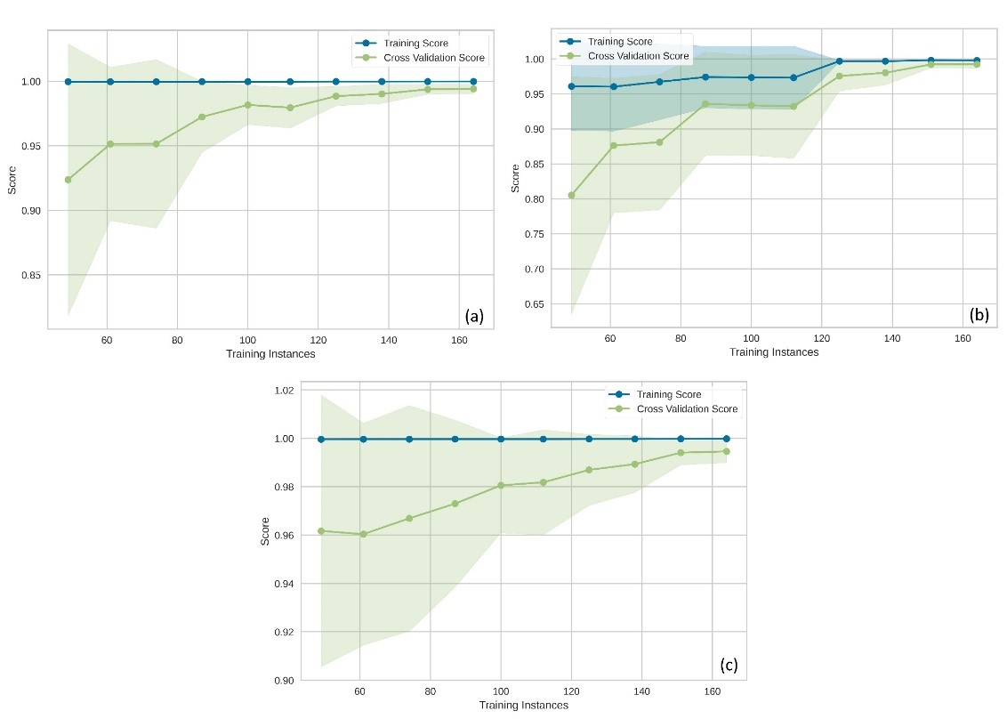
Figure 8. Learning curves (a) ETR with default hyperparameters, (b) ETR with tuned hyperparameters, and (c) VotingRegressor
As can be seen in Figure 8, the ETR with default hyperparameters reached 99 % convergence after 120 data instances and started to generalize the model. The standard deviations of the cross-validation results, shown as shaded green, also decreased after 100 data instances. On the other hand, the hyperparameter tuned ETR also reached an accurate calibration curve after 120 images. However, the final evaluation metrics were still not as good as untuned ETR. In addition, when this procedure was performed with less than 120 images, the training data score of the tuned ETR could not provide the desired values. When the learning curve of the blended model was examined in terms of mean cross-validation scores, it was seen that the blended model performed better than the untuned ETR model. The learning curves of the approaches showed that it is more reasonable to use VotingRegressor to construct an appropriate calibration curve.
In addition, prediction error plots were illustrated because an accurate estimate of the prediction error is mandatory to understand the final model (Frank, 2015). By referring to the 45-degree line, researchers have the privilege to diagnose regression models where the prediction exactly matches the model (Bengfort et al., 2018). The prediction error plots are shown below (Figure 9).
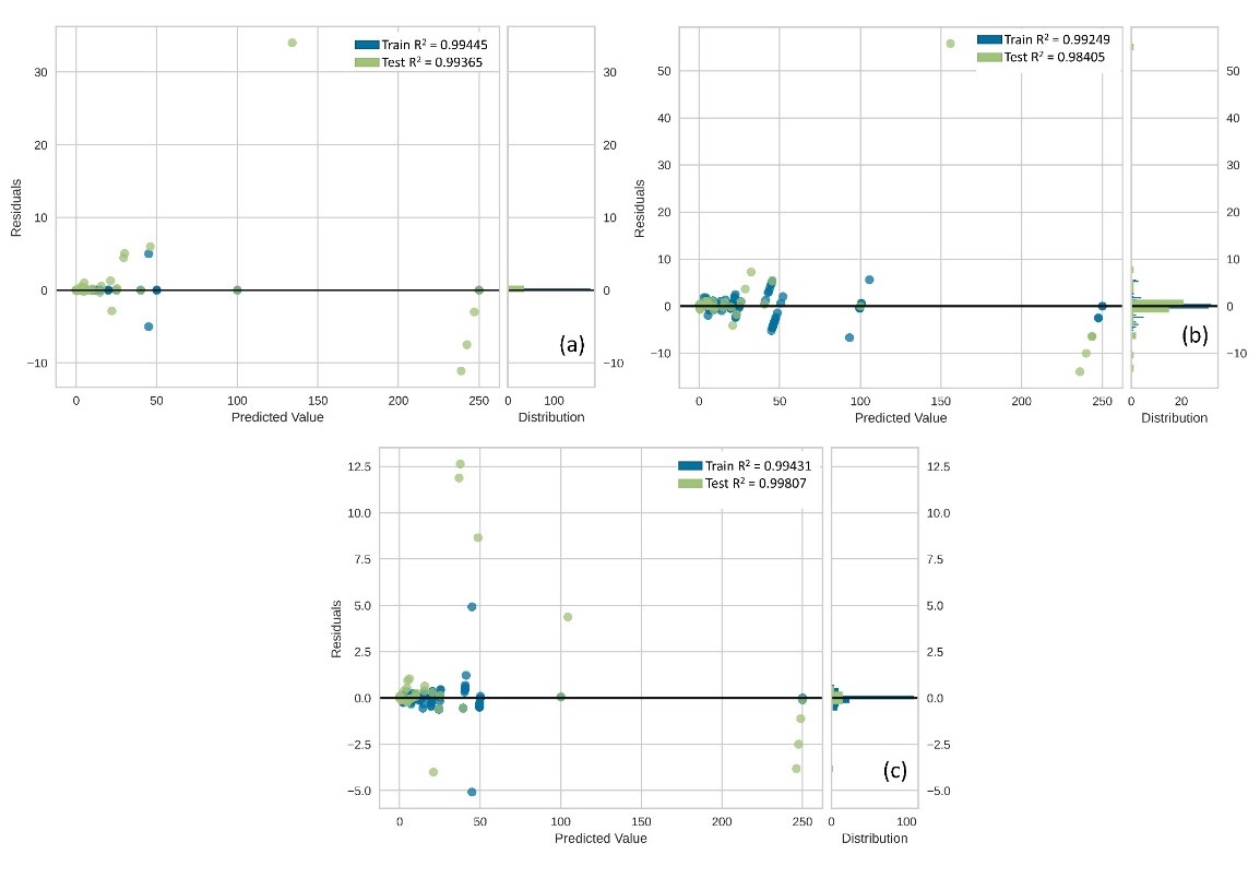
Figure 9. The prediction error plots (a) ETR with default hyperparameters, (b) ETR with tuned hyperparameters, and (c) VotingRegressor
When the prediction error plots were examined, it was visually confirmed that the validation results with the lowest variance were obtained with the Voting Regressor. Compared to the untuned ETR and the tuned ETR, the Voting Regressor estimated the ground truth more accurately for the 100 mg/L sample concentration. Finally, the residuals plot was drawn to see the residuals of the training data. The residuals plots for the three approaches are shown in Figure 10.
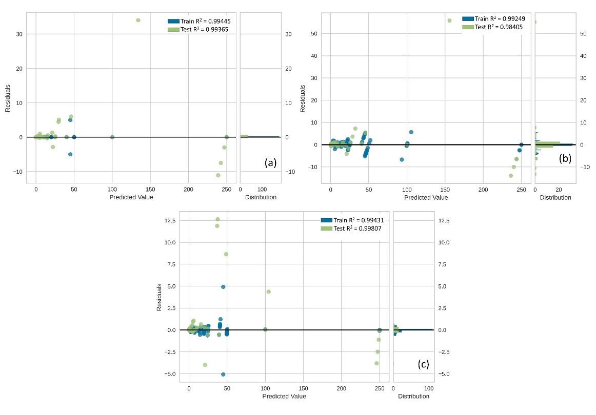
Figure 10. The residuals plots (a) ETR with default hyperparameters, (b) ETR with tuned hyperparameters, and (c) VotingRegressor
As seen in Figure 10(a), the default hyperparameter ETR model showed more bias in predicting high concentrations. The hyperparameter tuned ETR (Figure 10(b)) could not fully fit the training data into the regression process, which also explains why it had a lower training R2 value than other approaches. Figure 10(c) shows the residuals of the VotingRegressor. Compared to the untuned ETR, when VotingRegressor was used, the actual concentrations of the 100 mg/L and 250 mg/L samples converged, although there were more deviations at low concentrations (around 50 mg/L).
The models were then tested on the unseen data set (unknown samples for concentration measurement), which was never subjected to the regression process. The accuracy measures obtained are shown in Table 6.
Table 6. Testing models on unseen data
|
Accuracy Measures |
|||||
Model |
MAE |
MSE |
RMSE |
R2 |
RMSLE |
MAPE |
ETR with Default Hyperparameters |
0.19323 |
0.10564 |
0.32502 |
0.99975 |
0.05170 |
0.07630 |
ETR with Tuned Hyperparameters |
0.75212 |
1.38552 |
1.17695 |
0.99672 |
0.18519 |
0.70302 |
VotingRegressor |
0.26242 |
0.16586 |
0.40726 |
0.99961 |
0.07255 |
0.19135 |
Table 6 shows that even the accuracy measures of the default hyperparameter ETR is slightly better than VotingRegressor in estimating the concentration of unknown samples, the difference is negligible. Finally, the predicted concentrations of some of the unseen data by the models are given in Table 7.
Table 7. Predicted concentrations of some of the unseen data
Ground Truth |
Predicted Value |
||
ETR with Default Hyperparameters |
ETR with Tuned Hyperparameters |
VotingRegressor |
|
0.00 |
0.310 |
0.387 |
0.077 |
0.05 |
0.066 |
0.459 |
0.181 |
0.10 |
0.076 |
0.428 |
0.099 |
0.25 |
0.250 |
0.387 |
0.256 |
0.50 |
0.498 |
0.466 |
0.491 |
1.00 |
1.002 |
0.664 |
0.988 |
2.50 |
2.613 |
3.298 |
2.293 |
4.00 |
4.060 |
4.632 |
4.622 |
7.50 |
7.465 |
6.861 |
7.557 |
12.50 |
13.125 |
12.677 |
12.276 |
15.00 |
14.700 |
15.869 |
14.964 |
25.00 |
25.250 |
23.877 |
24.181 |
40.00 |
40.200 |
44.622 |
40.481 |
100.00 |
100.000 |
100.616 |
100.056 |
Naturally, the tuned hyperparameter ETR resulted in worse concentration estimates. The untuned ETR and the blended model predicted concentration values closer to the ground truth. The prediction results of the unseen data showed that visible spectrophotometry can be performed using the four-step procedure offered in the study. This work can be seen as a type of image regression. The best-known example of image regression is in age detection applications. The results suggest that a mobile application can be developed to measure the concentrations of colored samples using this procedure. With this application, concentration measurements can be carried out in laboratories or schools that cannot afford a spectrophotometer/colorimeter. Although the method presented is not currently suitable for analytical studies, it can be used in student experiments or situations where fast results are desired.
This method has several advantages, in addition to being mobile, providing rapid results and eliminating the need for traditional equipment. One of these is that this method does not require an adsorption spectrum to determine the wavelength of the sample. If the wavelength of the samples to be measured is unknown, a spectrum scan should be performed prior to the measurement. The absorbance spectrum is a plot of absorbance (A) versus wavelength (λ, in nm). The wavelength of a sample lies at the maximum λ value of the absorption spectrum curve (Marczenko and Balcerzak, 2000). This method avoids wasting time by skipping the wavelength scanning process. Another advantage of the presented method is that it is a closed procedure. This means that the necessary data set can be prepared by the researchers (the calibration curve (training data) unknown samples) and they can run this method without the need for external data input. In addition, if the background color of the images is the same as the solution to be measured, placing an A4 paper behind the solution can create a contrast with the background. In addition, speeding up the whole process or keeping the light source constant can be effective in providing more accurate concentration estimates. The photographs used in the study were taken under extremely modest conditions, and the only thing that was considered was not to block the ambient light during the photo shoot. There is therefore no reason why this method could not be repeated in other locations or under other lighting conditions. Although the photos used in this study were taken remotely using an application, the use of a Bluetooth selfie stick for remote photography can be considered as an alternative. Photographing the solutions without blocking the light intensity is very important for the accuracy of the whole process. However, it should not be forgotten that in traditional methods of analysis, the preparation of the standards and the samples are equally important for the accuracy of the measurement. Therefore, when using this method for different studies, it should be considered that incorrect results may be obtained due to random or systematic errors.
The study has some limitations. For example, the photographs used in the study were taken from only one angle (frontal) and with a fixed background of a different color to the color to be treated. The distance of the samples from the camera was 20, 30 and 40 cm, and whether this method will work with photos taken from further away is a new subject of research. In future research, the method will be developed into a mobile phone application.
4. Conclusion
This study investigated the estimation of the concentration of methylene blue solutions using smartphone photos and machine learning. The basic process sequence was to take photographs with remote photography, object detection and automatic ROI sampling with YOLOv5, find the dominant HSV code in the ROI, save the HSV codes with concentration value in a csv file and regression. 257 photographs of methylene blue solutions with concentrations varying from 0 - 250 mg/L were taken from distances of 20, 30, 40 cm. The test tubes in the photographs were detected using the pre-trained YOLOv5 object detection algorithm. The training process of YOLOv5 was performed with 928 enhanced images and the best mAP@05 value reached 0.915. After training, the detection process was performed on the images and 254 test tubes were detected in 257 images (99 %). With the modified detect.py file, the samples were simultaneously extracted from the ROI.
On the obtained samples, the HSV code of the most repeated color was determined, and the necessary csv file was prepared to be used in the regression process together with the concentration values. Among the 25 different regression algorithms, the model that reached the global optimum was the default hyperparameter extra trees regressor with a random state value of 449. The ETR training and validation R2 values were determined to be 99.5 % and 99.4 %, respectively. These results indicated that both a suitable calibration curve had been generated and that the model was not over- or under-fitting. A hyper-parameter tuning process of 3000 iterations was performed on ETR to improve the regression model. However, the desired accuracy measures were not achieved, and the fine-tuning process took a long time, which was contrary to one of the main objectives of the study. In a third approach to improve the accuracy measures, a VotingRegressor was created by combining the three best regressors (extra trees regressor, decision tree regressor and gradient boosting regressor). The accuracy measures of VotingRegressor were better than the default hyperparameter ETR, and when the learning curves were examined, VotingRegressor was better on the training data with fewer images. Low MAPE and MSE values in concentration estimation performed on unseen data for the default hyperparameter ETR and VotingRegressor showed that the presented method is very successful and can be used for non-scientific measurements. The results of this study prove that visible spectrophotometric analysis can be performed with a mobile phone application that includes object detection, sampling, dominant color finding and regression steps, respectively.
5. References
Ali, M., 2020. PyCaret: An open source, low-code machine learning library in Python. https://www.pycaret.org
Arabzadeh, V., Sohrabi, M. R., Goudarzi, N., & Davallo, M. (2019). Using artificial neural network and multivariate calibration methods for simultaneous spectrophotometric analysis of Emtricitabine and Tenofovir alafenamide fumarate in pharmaceutical formulation of HIV drug. Spectrochimica Acta Part A: Molecular And Biomolecular Spectroscopy, 215, 266-275. https://doi.org/10.1016/j.saa.2019.02.077
Aragaw, T. A., & Angerasa, F. T. (2020). Synthesis and characterization of Ethiopian kaolin for the removal of basic yellow (BY 28) dye from aqueous solution as a potential adsorbent. Heliyon, 6(9), e04975. https://doi.org/10.1016/j.heliyon.2020.e04975
Ariaeenejad, S., Motamedi, E., & Salekdeh, G. H. (2021). Application of the immobilized enzyme on magnetic graphene oxide nano-carrier as a versatile bi-functional tool for efficient removal of dye from water. Bioresource Technology, 319, 124228. https://doi.org/10.1016/j.biortech.2020.124228
Arpaia P., Azzopardi, G., Blanc, F., Bregliozzi, G., Buffat, X., Coyle, L., Fol, E., Giordano, F., Giovannozzi, M., Pieloni, T., Prevete, R., Redaelli, S., Salvachua, B., Salvant, B., Schenk, M., Camillocci, M. S., Tomás, R., Valentino, G., Van Der Veken, F. F., & Wenninger, J. (2021). Machine learning for beam dynamics studies at the CERN Large Hadron Collider. Nuclear Instruments And Methods In Physics Research Section A: Accelerators, Spectrometers, Detectors And Associated Equipment, 985, 164652. https://doi.org/10.1016/j.nima.2020.164652
Ayman, A., Zeid, A. M., Wahba, M. E. K., & El-Shabrawy, Y. (2020). Analysis of clozapine in its tablets using two novel spectrophotometric reactions targeting its tertiary amino group. Spectrochimica Acta Part A: Molecular And Biomolecular Spectroscopy, 238, 118447. https://doi.org/10.1016/j.saa.2020.118447
Aytaç, E. (2020). Unsupervised learning approach in defining the similarity of catchments: Hydrological response unit based k-means clustering, a demonstration on Western Black Sea Region of Turkey. International Soil And Water Conservation Research, 8(3), 321-331. https://doi.org/10.1016/j.iswcr.2020.05.002
Aytaç, E. (2021a). Forecasting Turkey’s Hazelnut Export Quantities with Facebook’s Prophet Algorithm and Box-Cox Transformation. Advances In Distributed Computing And Artificial Intelligence Journal, 10(1), 33-47. https://doi.org/10.14201/adcaij20211013347
Aytaç, E. (2021b). Havzaların benzerliklerini tanımlamada alternatif bir yaklaşım: hiyerarşik kümeleme yöntemi uygulaması. Fen Ve Mühendislik Bilimleri Dergisi, 21(4), 958-970. https://doi.org/10.35414/akufemubid.870649
Aytaç, E. (2022a). Exploring Electrocoagulation Through Data Analysis and Text Mining Perspectives. Environmental Engineering And Management Journal, 21(4), 317-331.
Aytaç E. (2022b). Modeling Future Impacts on Land Cover of Rapid Expansion of Hazelnut Orchards: A Case Study on Samsun, Turkey. European Journal Of Sustainable Development Research, 6(4), em0193. https://doi.org/10.21601/ejosdr/12167
Aytaç, E., Fombona‐Pascual, A., Lado, J. J., García-Quismondo, E., Palma, J., & Khayet, M. (2023d). Faradaic deionization technology: Insights from bibliometric, data mining and machine learning approaches. Desalination, 563, 116715. https://doi.org/10.1016/j.desal.2023.116715
Aytaç, E., & Khayet, M., (2023a). Machine Learning Applications on Membrane Distillation. Fourteen International Conference on Thermal Engineering: Theory and Applications, May 25-27, Yalova, Türkiye.
Aytaç, E., & Khayet, M. (2023b). A deep dive into membrane distillation literature with data analysis, bibliometric methods, and machine learning. Desalination, 553, 116482. https://doi.org/10.1016/j.desal.2023.116482
Aytaç E., & Khayet, M. (2023c). A Topic Modeling Approach to Discover the Global and Local Subjects in Membrane Distillation Separation Process. Separations, 10(9), 482. https://doi.org/10.3390/separations10090482
Azimi, M., & Pacut, A. (2020). Investigation into the reliability of facial recognition systems under the simultaneous influences of mood variation and makeup. Computers & Electrical Engineering, 85, 106662. https://doi.org/10.1016/j.compeleceng.2020.106662
Bengfort, B., Bilbro, R., McIntyre, K., Gray, L., Roman, P., Morris, A., & Danielsen, N. (2018). Yellowbrick.
Bora, D. J., Gupta, A. K., & Khan, F. A. (2015). Comparing the Performance of L*A*B* and HSV Color Spaces with Respect to Color Image Segmentation. Paper presented at the International Journal of Emerging Technology and Advanced Engineering.
Bunnag, N., Kasri, B., Setwong, W., Sirisurawong, E., Chotsawat, M., Chirawatkul, P., & Saiyasombat, C. (2020). Study of Fe ions in aquamarine and the effect of dichroism as seen using UV–Vis, NIR and x-ray. Radiation Physics And Chemistry, 177, 109107. https://doi.org/10.1016/j.radphyschem.2020.109107
Cardani, D. (2001). Adventures in HSV Space. http://robotlab.itk.ppke.hu/~rakadam/hsvspace.pdf
Chen, S. J., Karabucak, B., Steffen, J. J., Yu, Y., & Kohli, M. R. (2020). Spectrophotometric Analysis of Coronal Tooth Discoloration Induced by Tricalcium Silicate Cements in the Presence of Blood. Journal Of Endodontics, 46(12), 1913-1919. https://doi.org/10.1016/j.joen.2020.09.009
Chen, Y., & Miao, D. (2020). Granular regression with a gradient descent method. Information Sciences, 537, 246-260. https://doi.org/10.1016/j.ins.2020.05.101
Cheng, H., Li, H., Dia, Q., and Yang, J., 2023. A deep reinforcement learning method to control chaos synchronization between two identical chaotic systems. Chaos, Solitons & Fractals, 174: 113809. doi: https://doi.org/10.1016/j.chaos.2023.113809
Chung, S., Park, Y. W., & Cheong, T. (2020). A mathematical programming approach for integrated multiple linear regression subset selection and validation. Pattern Recognition, 108, 107565. https://doi.org/10.1016/j.patcog.2020.107565
Claudino, D., Ricci, W. A., Honório, H., Machry, R. V., Valandro, L. F., Da Rosa, R. A., & Pereira, J. R. (2021). Spectrophotometric analysis of dental bleaching after bonding and debonding of orthodontic brackets. The Saudi Dental Journal, 33(7), 650-655. https://doi.org/10.1016/j.sdentj.2020.05.003
Danchana, K., De Souza, C. T., Palacio, E., & Cerdà, V. (2019). Multisyringe flow injection analysis for the spectrophotometric determination of uranium (VI) with 2-(5-bromo-2-pyridylazo)-5-diethylaminophenol. Microchemical Journal, 150, 104148. https://doi.org/10.1016/j.microc.2019.104148
De Carvalho, F. d. A. T., Lima Neto, E. d. A., & Da Silva, K. C. F. (2021). A clusterwise nonlinear regression algorithm for interval-valued data. Information Sciences, 555, 357-385. https://doi.org/10.1016/j.ins.2020.10.054
Dogan, A., & Birant, D. (2021). Machine learning and data mining in manufacturing. Expert Systems With Applications, 166, 114060. https://doi.org/10.1016/j.eswa.2020.114060
Dumancas, G. G., Bello, G., Sevilleno, S., Subong, B. J. J., Koralege, R. H., Nuwan Perera, U. D & Goudelock, A. (2017). Spectrophotometric Analysis of Food Colorants. In Reference Module in Food Science: Elsevier. https://doi.org/10.1016/B978-0-08-100596-5.21457-1
Duysak, H., & Yigit, E. (2020). Machine learning based quantity measurement method for grain silos. Measurement, 152, 107279. https://doi.org/10.1016/j.measurement.2019.107279
Ebraheem, S. A. M., Elbashir, A. A., & Aboul‐Enein, H. Y. (2011). Spectrophotometric methods for the determination of gemifloxacin in pharmaceutical formulations. Acta Pharmaceutica Sinica B, 1(4), 248-253. https://doi.org/10.1016/j.apsb.2011.10.005
Eyring, M. B. (2003). Spectroscopy in Forensic Science. In R. A. Meyers (Ed.), Encyclopedia of Physical Science and Technology (Third Edition) (pp. 637-643). New York: Academic Press. https://doi.org/10.1016/B0-12-227410-5/00957-1
Frank, E., & Harrell, J. (2015). Regression Modeling Strategies. Switzerland: Springer, Cham. https://doi.org/10.1007/978-3-319-19425-7
García-González, A., Zavala-Arce, R. E., Ávila-Pérez, P., Jiménez‐Núñez, M. L., García-Gaitán, B., & García-Rivas, J. L. (2020). Development of standardized method for the quantification of azo dyes by UV-Vis in binary mixtures. Analytical Biochemistry, 608, 113897. https://doi.org/10.1016/j.ab.2020.113897
García-Lamont, F., Cervantes, J., López, A., & Rodríguez, L. (2018). Segmentation of images by color features: A survey. Neurocomputing, 292, 1-27. https://doi.org/10.1016/j.neucom.2018.01.091
Guha, A., Lei, R., Zhu, J., Nguyen, X., & Zhao, D. (2022). Robust unsupervised learning of temporal dynamic vehicle-to-vehicle interactions. Transportation Research Part C: Emerging Technologies, 142, 103768. https://doi.org/10.1016/j.trc.2022.103768
Hao, Z., Jin, L., Lyu, R., & Akram, H. R. (2020). Problematic mobile phone use and altruism in Chinese undergraduate students: The mediation effects of alexithymia and empathy. Children And Youth Services Review, 118, 105402. https://doi.org/10.1016/j.childyouth.2020.105402
Huong, D. T. M., Chai, W. S., Show, P. L., Lin, Y., Chiu, C., Tsai, S., & Chang, Y. (2020). Removal of cationic dye waste by nanofiber membrane immobilized with waste proteins. International Journal Of Biological Macromolecules, 164, 3873-3884. https://doi.org/10.1016/j.ijbiomac.2020.09.020
Jocher, G., Stoken, A., Borovec, J., NanoCode012, ChristopherSTAN, Changyu, L., & Yu, L. (2021). ultralytics/yolov5: v4.0 - nn.SiLU() activations, Weights \and Biases logging, PyTorch Hub integration (Version v4.0): Zenodo. https://doi.org/10.5281/zenodo.4418161
Jung, A. B. (2018). imgaug. https://github.com/aleju/imgaug
Kandi, S., & Charles, A. L. (2019). Statistical comparative study between the conventional DPPH spectrophotometric and dropping DPPH analytical method without spectrophotometer: Evaluation for the advancement of antioxidant activity analysis. Food Chemistry, 287, 338-345. https://doi.org/10.1016/j.foodchem.2019.02.110
Khayet, M., Aytaç, E., & Matsuura, T. (2022). Bibliometric and sentiment analysis with machine learning on the scientific contribution of Professor Srinivasa Sourirajan. Desalination, 543, 116095. https://doi.org/10.1016/j.desal.2022.116095
Kukielski, M., Kędzierska-Sar, A., Kuś, S., Wiecińska, P., & Szafran, M. (2019). Application of highly sensitive spectrophotometric analysis in detection of metal content in molybdenum reinforced alumina obtained by precursor infiltration of ceramic preforms. Ceramics International, 45(17), 22047-22054. https://doi.org/10.1016/j.ceramint.2019.07.221
Lian, W., Chao, H., Shuping, Z., Jinkai, L., Jianchuan, Z., Zhongwei, C., Zhen, Y., Yong, X., & Min, Z. (2023). Robust fall detection in video surveillance based on weakly supervised learning. Neural Networks, 163, 286-297. https://doi.org/10.1016/j.neunet.2023.03.042
Liu, G., Han, J., & Rong, W. (2021). Feedback-driven loss function for small object detection. Image And Vision Computing, 111, 104197. https://doi.org/10.1016/j.imavis.2021.104197
Liu, Y., Mazumdar, S., & Bath, P. A. (2023). An unsupervised learning approach to diagnosing Alzheimer’s disease using brain magnetic resonance imaging scans. International Journal Of Medical Informatics, 173, 105027. https://doi.org/10.1016/j.ijmedinf.2023.105027
Marczenko, Z., & Balcerzak, M. (2000). Separation, Preconcentration and Spectrophotometry in Inorganic Analysis. In E. Kloczko (Ed.), Analytical Spectroscopy Library (1st ed., Vol. 10, pp. 39-52): Elsevier Science.
Masawat, P., Harfield, A., & Namwong, A. (2015). An iPhone-based digital image colorimeter for detecting tetracycline in milk. Food Chemistry, 184, 23-29. https://doi.org/10.1016/j.foodchem.2015.03.089
Meek, C., Thiesson, B., & Heckerman, D. (2002). The Learning-Curve Sampling Method Applied to Model-Based Clustering. Journal of Machine Learning Research, 2, 397-418.
Mijinyawa, A. H., Mishra, A., & Durga, G. (2020). Cationic dye removal using a newer material fabricated by Taro Mucilage-g-PLA and Organobentonite clay. Materials Today: Proceedings. https://doi.org/10.1016/j.matpr.2019.12.345
Milojevic-Dupont, N., & Creutzig, F. (2021). Machine learning for geographically differentiated climate change mitigation in urban areas. Sustainable Cities And Society, 64, 102526. https://doi.org/10.1016/j.scs.2020.102526
Mokhtari, N., Afshari, M., & Dinari, M. (2020). Synthesis and characterization of a novel fluorene-based covalent triazine framework as a chemical adsorbent for highly efficient dye removal. Polymer, 195, 122430. https://doi.org/10.1016/j.polymer.2020.122430
Nguyen, T., Roy, A., & Memon, N. (2019). Kid on the phone! Toward automatic detection of children on mobile devices. Computers & Security, 84, 334-348. https://doi.org/10.1016/j.cose.2019.04.001
Osarogiagbon, A. U., Khan, F., Venkatesan, R., & Gillard, P. (2021). Review and analysis of supervised machine learning algorithms for hazardous events in drilling operations. Process Safety And Environmental Protection, 147, 367-384. https://doi.org/10.1016/j.psep.2020.09.038
Pal, P., Corpuz, A. G., Hasan, S. W., Sillanpää, M., & Banat, F. (2021). Simultaneous removal of single and mixed cationic/anionic dyes from aqueous solutions using flotation by colloidal gas aphrons. Separation and Purification Technology, 255: 117684. https://doi.org/10.1016/j.seppur.2020.117684
Pedregosa, F., Varoquaux, G., Gramfort, A., Michel, V., Thirion, B., Grisel, O., & Duchesnay, E. (2011). Scikit-learn: Machine Learning in {P}ython. Journal of Machine Learning Research, 12(85): 2825-2830.
Pereda, M., & Estrada, E. (2019). Visualization and machine learning analysis of complex networks in hyperspherical space. Pattern Recognition, 86, 320-331. https://doi.org/10.1016/j.patcog.2018.09.018
Perroni, A. P., Bergoli, C. D., dos Santos, M. B. F., Moraes, R. R., & Boscato, N. (2017). Spectrophotometric analysis of clinical factors related to the color of ceramic restorations: A pilot study. The Journal Of Prosthetic Dentistry, 118(5): 611-616. https://doi.org/10.1016/j.prosdent.2016.12.010
Pradhan, S. S., Konwar, K., Ghosh, T. N., Mondal, B., Sarkar, S. K., & Deb, P. (2020). Multifunctional Iron oxide embedded reduced graphene oxide as a versatile adsorbent candidate for effectual arsenic and dye removal. Colloid And Interface Science Communications, 39, 100319. https://doi.org/10.1016/j.colcom.2020.100319
Priya, Sharma, A. K., Kaith, B. S., Chandel, K., Vipula, Isha, & Singh, A. (2020). Bifunctional gelatin/dextrin hybrid backbone based fluorescent chemo-sensor for the detection of tannic acid and removal of eosin yellow dye. Materials Chemistry And Physics, 254, 123304. https://doi.org/10.1016/j.matchemphys.2020.123304
Ragab, M. A. A., El Yazbi, F. A., Hassan, E. M., Khamis, E. F., & Hamdy, M. M. A. (2018). Spectrophotometric analysis of two eye preparations, vial and drops, containing ketorolac tromethamine and phenylephrine hydrochloride binary mixture and their ternary mixture with chlorphenirmaine maleate. Bulletin Of Faculty Of Pharmacy, Cairo University, 56(1), 91-100. https://doi.org/10.1016/j.bfopcu.2018.03.004
Shuang, K., Lyu, Z., Loo, J., & Zhang, W. (2021). Scale-balanced loss for object detection. Pattern Recognition, 117, 107997. https://doi.org/10.1016/j.patcog.2021.107997
Sliney, D. H. (2016). What is light? The visible spectrum and beyond. Eye, 30(2), 222-229. https://doi.org/10.1038/eye.2015.252
Solovyev, R., Wang, W., & Gabruseva, T. (2021). Weighted boxes fusion: Ensembling boxes from different object detection models. Image And Vision Computing, 107, 104117. https://doi.org/10.1016/j.imavis.2021.104117
Soni, S., Bajpai, P. K., Mittal, J., & Arora, C. (2020). Utilisation of cobalt doped Iron based MOF for enhanced removal and recovery of methylene blue dye from waste water. Journal Of Molecular Liquids, 314, 113642. https://doi.org/10.1016/j.molliq.2020.113642
Sumriddetchkajorn, S., Chaitavon, K., & Intaravanne, Y. (2013). Mobile device-based self-referencing colorimeter for monitoring chlorine concentration in water. Sensors And Actuators B: Chemical, 182, 592-597. https://doi.org/10.1016/j.snb.2013.03.080
Sun, G., Wen, Y., & Yu, L. (2022). Instance segmentation using semi-supervised learning for fire recognition. Heliyon, 8(12), e12375. https://doi.org/10.1016/j.heliyon.2022.e12375
Sural, S., Gang, Q., & Pramanik, S. (2002). Segmentation and histogram generation using the HSV color space for image retrieval. Paper presented at the Proceedings. International Conference on Image Processing.
Turchioe, M. R., Jimenez, V., Isaac, S., Alshalabi, M., Slotwiner, D., & Creber, R. M. (2020). Review of mobile applications for the detection and management of atrial fibrillation. Heart Rhythm O2, 1(1), 35-43. https://doi.org/10.1016/j.hroo.2020.02.005
Vishwakarma, R., & Vennelakanti, R. (2020). CNN Model and Tuning for Global Road Damage Detection. Paper presented at the 2020 IEEE International Conference on Big Data (Big Data), Los Alamitos, CA, USA. https://doi.org/10.1109/BigData50022.2020.9377902
Wang, R.-F., Deng, L.-G., Li, K., Fan, X.-J., Li, W., & Lu, H.-Q. (2020). Fabrication and characterization of sugarcane bagasse–calcium carbonate composite for the efficient removal of crystal violet dye from wastewater. Ceramics International, 46(17), 27484-27492. https://doi.org/10.1016/j.ceramint.2020.07.237
Yap, M. H., Hachiuma, R., Alavi, A., Brungel, R., Goyal, M., Zhu, H., & Frank, E. (2020). Deep Learning in Diabetic Foot Ulcers Detection: A Comprehensive Evaluation. ArXiv, abs/2010.03341.
Yuan, W., & Rui, X. (2023). Deep reinforcement learning-based controller for dynamic positioning of an unmanned surface vehicle. Computers & Electrical Engineering, 110, 108858. https://doi.org/10.1016/j.compeleceng.2023.108858
Zayed, M. A., Imam, N. G., Ahmed, M. A., & El Sherbiny, D. H. (2017). Spectrophotometric analysis of hematite/magnetite nanocomposites in comparison with EDX and XRF techniques. Journal Of Molecular Liquids, 231, 288-295. https://doi.org/10.1016/j.molliq.2017.02.007
Ziaei, F., & Ranjbar, M. 2023. A reinforcement learning algorithm for scheduling parallel processors with identical speedup functions. Machine Learning with Applications, 155, 100485. https://doi.org/10.1016/j.mlwa.2023.100485
Zualkernan, I., Aloul, F., Shapsough, S., Hesham, A., & El-Khorzaty, Y. (2017). Emotion recognition using mobile phones. Computers & Electrical Engineering, 60, 1-13. https://doi.org/10.1016/j.compeleceng.2017.05.004