ADCAIJ: Advances in Distributed Computing and Artificial Intelligence Journal
Regular Issue, Vol. 11 N. 4 (2022), 427-450
eISSN: 2255-2863
DOI: https://doi.org/10.14201/adcaij.28394
Analyzing Social Media Sentiment: Twitter as a Case Study
Yaser A. Jasima, Mustafa G. Saeedb and Manaf B. Raewfc
aDepartment of Accounting, Cihan University-Erbil, Kurdistan Region, Iraq.
bDepartment of Computer Science, Cihan University Sulaimanyia, Sulaimanyia, 46001, Kurdistan Region, Iraq.
cDepartment of Human Resource Management, Cihan University-Erbil, Kurdistan Region, Iraq.
yaser.jasim@cihanuniversity.edu.iq, mostafa.swe@gmail.com, manaf.basil@cihanuniversity.edu.iq
ABSTRACT
This study examines the problem of Twitter sentiment analysis, which categorizes Tweets as positive or negative. Many applications require the analysis of public mood, including organizations attempting to determine the market response to their products, political election forecasting, and macroeconomic phenomena such as stock exchange forecasting. Twitter is a social networking microblogging and digital platform that allows users to update their status in a maximum of 140 characters. It is a rapidly expanding platform with over 200 million registered profiles and 100 million active users. Half of Twitter’s active users log on daily, tweeting over 250 million tweets. Public opinion analysis is critical for applications, including firms looking to understand market responses to their products, predict political choices, and forecast socio-economic phenomena such as bonds. Through deep learning methodologies, a recurrent neural network with convolutional neural network models was constructed for Twitter sentiment analysis to predict if a tweet is positive or negative using a dataset of tweets. The applied methods were trained via a publicly available dataset of 1,600,000 tweets. Several model architectures were trained, with the best achieving a (93.91%) success rate in recognizing the tweets' matching sentiment. The model's high success rate makes it a valuable advisor and a technique that might be improved to enable an integrated sentiment analyzer system that can work in real-world situations for political marketing.
KEYWORDS
deep learning; artificial intelligence; social media; data modeling; Twitter; CNN
1. Introduction
Pattern classification and data mining are two concepts that are very closely connected and may be described officially as a process, either unsupervised or supervised, identifying relevant patterns in a large amount of data. Sentiment analysis has gained prominence in research as it enables understanding individuals' thoughts on an issue through the evaluation of big data. Many individuals utilize social networking sites, forums, and commonplace review websites to offer their perspectives on various services or goods. Obtaining active feedback from individuals is significant, not just for businesses measuring customer loyalty and competitors, but also for consumers who prefer to research a product or service before making a purchase (Abdullah and Mohammed, 2019) (Deborah et al., 2021).
Subjectivity and Sentiment Analysis (SSA) has garnered considerable attention in recent years because of its importance in marketing and politics. A subjectivity classification is the classification of texts as objective or subjective. The sentiment categorization tool detects whether a subjective text is good, bad, unbiased, or mixed (Elnagar et al., 2021). These many forms of SSA are becoming more prevalent because they give an automatic means of summarizing enormous quantities of text (review sites, forums, and Twitter feeds) into the conveyed ideas. Because of the broad availability of social media platforms, anyone may share their views or opinions about an occurrence, product, or problem (Niloufar et al., 2021). Mining these informal and homogenous data is critical for making conclusions in fields. However, mining is challenging due to the massively unstructured nature of the sentiment data available on the web (Govindarajan, 2021). On the internet, textual information is divided into two categories: fact data and sentiment data (Xipeng et al., 2020); By extracting important patterns and characteristics from a large dataset of tweets, the paper mainly relies on natural language processing techniques; and machine learning techniques to identify individual training dataset samples (tweets) based on the pattern model that best represents data.
Sentiment analysis offers a wide range of applications. The capacity to learn from social data is widely used in business. The following are some notable areas of sentiment analysis: Social media opinion analysis, social discussions in their social environment, and sentiment from the audience. Although businesses must track their mentions, sentiment analysis delves into the good, bad, and neutrals, as well as what individuals think about the company's goods or services (Mohammed, 2019) (Thabit and Jasim, 2017). However, sentiment analysis enables someone to monitor consumer reactions to the specific features of a product. This method might be carried out by monitoring general public sentiment toward that business over time and using economic tools to evaluate the link between public sentiment and the firm's stock market valuation (Thabit and Yaser, 2017).
The purpose of this paper is to examine the topic of sentiment analysis on Twitter. Whereas, tweets are classified based on whether they express a good, bad, or neutral attitude. Twitter is a microblogging and social networking website where users may submit 140-character status updates (Geetika and Yadav, 2014). This process is a fast-developing site, with over 200 million registered users, where 100 million users are active users, with half of them logging on daily, resulting in almost 250 million tweets daily. The authors aim to establish a representation of public opinion for decision-making by studying the emotions conveyed in tweets (Juan, 2021). Analyzing public opinion is essential for a variety of reasons, including corporations seeking to anticipate customer reactions to their products, forecasting political elections, and anticipating socioeconomic events such as the stock exchange. This work seeks to develop a practical classifier based on long short-term memory (LSTM) in the field of deep learning that can reliably and automatically assess the sentiment of an unknown Twitter stream (Alexander, 2019).
2. Related Works
In recent years, a considerable amount of research has been conducted on sentiment analysis. The strategy proposed by Chen et al. (2014) classified student data into several categories and solved student issues reported on Twitter (Peng et al., 2017). As Bhilare and Kasture argued, to mine opinions posted on social media sites, it is necessary to know grammar, how tags work, vocabulary, and semantic networks (Neethu and Rajasree, 2013), which covers sentiment classification and data collection methods (Sagar et al., 2014). In the domain of electronic goods, the accuracy of the classification technique using the specified feature vector and several classifiers, such as maximum probability, support vector machine, and ensemble classifiers, was investigated (Neha and Bhilare, 2015). The authors described a hybrid technique for identifying polarity in subjective consumer-product texts that incorporates sentiment lexicons and a machine-learning classifier (Seyed-Ali and Andreas, 2013). Gautam and Yadav (2014) provided a set of machine learning algorithms with semantic analysis to detect phrases and product evaluations based on Twitter data using WordNet for higher accuracy (Geetika and Yadav, 2014). Gokulakrishnan et al. evaluated the output of several classifiers for Twitter data categorization, such as social media optimization (SMO), SVM, and Random Forest (Balakrishnan et al., 2012). The authors proposed a method for normalizing noisy or nonsensical tweets and classifying them according to polarity, in other words, positive or negative. They also utilized a mixed model technique to generate numerous emotional words (Asil et al., 2010).
3. Sentiment Analysis
Sentiment analysis, commonly referred to as opinion mining or emotion AI, is indeed the systematic recognition, extraction, assessment, and evaluation of emotional responses and opinions of the respondents utilizing natural language processing (NLP), text mining, machine learning, and biometrics. The voice in client materials, such as online surveys and reviews, as well as web-based social networking sites, is the primary focus of sentiment analysis (Abdullah, A. and Faisal, 2017). Sentiment analysis, in general, aims to analyze the attitude of a speaker, author, or other subjects in terms of topic, by noticing powerful psychological or intense reactions to an archive, conversation, or incident (Jasim and Mustafa, 2018). The attitude seems to be an emotional decision or evaluation, such as the creator's or presenter's passionate condition or an expectation of enthusiastic responses, in other words, the author's or dealer's intended impact.
User evaluations or comments on a broad range of concerns are already widely available on the Internet, and inspections may provide, among other things, user or media fault-finding questionnaires (Mustafa et al., 2021). Surveys are becoming increasingly popular as individuals seek to express themselves online. As a result, there are a significant number of surveys accessible for every topic, making it difficult for users to decide which one to take, as they must read each one before deciding. A sentiment's polarity can be categorized as positive, negative, or neutral. It is indeed essential to mention that emotion mining may be done on three different levels (Nik et al., 2020):
1. Document-level sentiment classification: At this level, a document can be classed entirely as positive, negative, or neutral.
2. Sentence-level sentiment classification: At this level, each statement is graded as good, negative, or impartial.
3. Aspect and feature level sentiment classification: At this level, sentences/documents can be labeled as positive, negative, or non-partisan depending on particular features of the sentences/archives, a process known as perspective-level evaluation grouping.
Central to the discipline of sentiment analysis is numerical representations of words, phrases, or documents. When using machine learning or deep learning techniques in text classification problems, the input characteristics used to represent text data in the model are word representations or word embedding (Muhamad et al., 2021). There are various forms of representations: one-hot, bag-of-words, word2vec, fast text, glove, word embedding, and others (Judith et al, 2017). As a consequence, mining this data and separating and organizing customer reviews is a responsibility. Sentiment mining is a work that involves scanning a huge number of archives with natural language processing (NLP) and information extraction (IE) techniques to synthesize the sentiments in the remarks of various authors (Andreas et al., 2017). In this approach, two techniques are used: computational etymology and information retrieval (IR). The basic idea underlying sentiment analysis is to assess the polarity of text documents or short phrases and then categorize them (Christopher, 2020).
4. Word Embedding
Using a word embedding model to turn all words into a real-valued vector is one method of expressing a text numerically. Word embedding is a high-dimensional vector produced by word mapping with a parameterized function developed using a data set typical of the source language. Word embedding enables the mapping of related words to the same location, which is a significant advantage. The t-distributed stochastic neighbor embedding (t-SNE) is a probabilistic approach for dimensionality reduction that may be used to display high-dimensional datasets, such as word embedding (Christopher, 2020).
In Figure 1, the similarities between data points are converted into joint probabilities using t-SNE. Furthermore, the t-SNE tries to decrease the disparity between high-dimensional data and joint probabilities (Matthew et al., 2020). Since the dimensionality is reduced, axes and their units on t-SNE plots have no meaningful relevance; however, t-SNE displays which point is closest to the source domain. Figure 1 shows a zoomed-in view of the quantity and the job regions in the t-SNE visual developed using word embedding as an example of bene t. In addition, there are four basic types of embedding: word2vec algorithms, glove, and embedding layer learning, as well as deep learning. The embedding layer was employed in this study to represent the words as vectors, and this layer was learned using the deep learning model ((Nik et al., 2020).
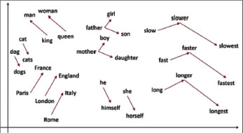
Figure. 1. t-SNE of Word Embedding
4.1. Embedding Layer
As a consequence, a layer is created to translate the one-hot representations into word embedding, and given a series of T words {w1, w2,…., wT}, each word wt ∈ W is embedded into a word-dimensional vector space using the following Equation as 1:
The matrix 𝐄 ∈ ℝdwrdd×|𝒲|, as the other network's other parameters, represents all of the word embedding to be learned in this layer. In reality, the authors employ a lookup table to replace this computation with a more basic array indexing operation, where Ewt ∈ ℝdwrd relates to the word wt embedding. This lookup table action is then performed on each word in the sequence. A popular strategy is to concatenate all of the resultant word embeddings, as illustrated in Equation 2; this vector may then be given to further neural network layers (Mohammed and Jose, 2020).
5. Deep Learning
Deep learning is a subclass of machine learning that uses multi-layer Neural Networks to transmit data from input to output and achieve improved accuracy in translation, speech recognition, and detection (Rohit, 2018), as seen in Figure 2.
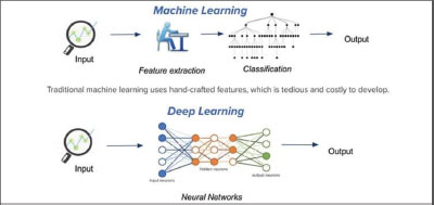
Figure. 2. Difference between ML and DL
Deep Learning differs from traditional ML methodologies. It can learn characteristics from data, such as photos, video, or text, autonomously, with no intervention from humans or implicitly supplied actions (Jan et al, 2021). When additional data is provided, the architectures of Neural Networks (NNs) may improve their prediction accuracy by directly learning from the raw data. DL is responsible for a variety of innovative developments, including voice assistants and self-driving automobiles (Rohit, 2018).
6. Types of Deep Learning Algorithms and Techniques
Deep Learning techniques are classed as unsupervised, supervised, partially supervised, or semi-supervised. Another form of learning approach known as Reinforcement Learning (RL) or Deep Reinforcement Learning (DRL) is occasionally contested inside semi-supervised or frequently within unsupervised learning techniques (Priyanka and Silakari, 2021).
6.1. Deep Supervised Learning
Deep Supervised Learning makes use of labeled data. In this category, the environment has a set of inputs and equivalent outputs. For example, if the intelligent agent forecasts for input xt, the agent obtains loss values. Following that, the agent iteratively changes the network parameters to obtain more adequate approximations for desired output values. During practical training, the agent can ensure accurate responses to inquiries posed by the environment. There are several supervised learning algorithms for DL, including Convolutional Neural Networks (CNNs), Deep Neural Networks (DNNs), and Recurrent Neural Networks (RNNs), which use Long Short-Term Memory (LSTM) and Gated Recurrent Units (GRUs) (Fahad et al., 2020) (Nasim et al., 2019).
6.2. Deep Semi-Supervised Learning
Deep semi-supervised learning occurs using partially labeled datasets. As semi-supervised learning algorithms, for example, Generative adversarial networks (GANs) and Deep Reinforcement Learning are used. RNNs, such as GRU and LSTM, were also used for semi-supervised learning (Ajay and Ausif, 2019) (Manuel et al., 2021).
6.3. Deep Unsupervised Learning
Deep unsupervised learning is capable of doing so in the absence of data labels. In this situation, the agent will learn crucial characteristics or internal models to identify new correlations or structures in input data (Thabit and Yaser, 2015). Dimensionality reduction and clustering algorithms are also referred to as unsupervised learning techniques. Furthermore, several DL family members, such as GAN, Restricted Boltzmann Machines (RBMs), and Auto-Encoders (AE), specialize in clustering and nonlinear dimensionality reduction; recurrent neural networks, such as RL and LSTM, are also used for unsupervised learning in a variety of application areas (Marina and Emanuele, 2020).
7. Recurrent Neural Network
A recurrent neural network (RNN) is a kind of NN in which the connections between neurons produce a single directed cycle, as shown in Figure 3. Because sentences are a collection of words and documents, this feature is useful in NLP. RNNs are called recurrent because they conduct the same operations in each element (Yaser et al., 2021). Furthermore, RNNs may remember the information they have seen in the sequence. However, they can only reflect a few steps in training, making them unsuitable for modeling long-term dependencies; This has a diminishing curve problem. To address this problem, most applications employ a specifically built RNN known as LSTM, which is significantly less vulnerable to these concerns (Marina and Emanuele, 2020).
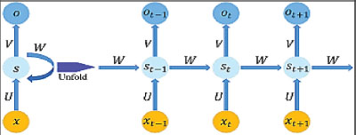
Figure. 3. A Simple RNN Architecture
7.1. Long Short-Term Memory
A long short-term memory is primarily an advanced RNN that is less vulnerable to the diminishing curve problem, and also better capable of analyzing long-distance relationships in sequence; these features make it useful for NLP applications where sentences and documents are sequential in nature (Yaser, 2018). LSTM is only intended to memorize a portion of the sequence observed thus far as illustrated in Figure 4. This behavior may be performed using network gates to determine what to store in memory depending on the current input and concealed state (Jasim and Mustafa, 2018).
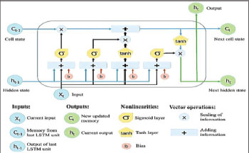
Figure. 4. The Basic Architecture of an LSTM Cell
The same effect occurs so often in separate time. It describes the governing in LSTM Equations (3-8):
Where it = input gate at time-step t; ot representing the output gate at time-step t; ft representing the forget gate at time-step t; Cin representing the value of candidate state at time-step t; Ct representing the state of the cell at time-step t; and ht represents hidden LSTM cell output at time-step t. In contrast, the gate values are based on the current input and output regarding the preceding cell. Indicating the previous and current information for making decisions about that to keep in memory.
A new cell memory is developed in equation 5 by discarding a portion of the present memory and absorbing some recent input xt. In equation 8, the LSTM cell produces a portion of the new memory as output, however, the last cell output is normally treated as the final output, reflecting the full sequence. Within a few instances, a version related to LSTM known as peephole LSTM was used. The distinction is that the gates are based on the value of the preceding cell rather than the output of the previous cell (Alexander, 2019).
7.2. Activation Function Type in Deep Learning
The activation function is critical in the architecture of ANN models. The activation function applies a nonlinear adjustment to the input signal to learn and do more complex nonlinear tasks. Nonlinear activation functions are often utilized in neural networks. Sigmoid functions, Rectified Linear Unit (ReLU), and hyperbolic tangent (tanh) are the most widely employed activation functions (Chigozie et al., 2018). The sigmoid function, often known as the logistic function, is a commonly used activation function. It is defined as a monotonically growing function in Equation 9:
7.2.1. Sigmoid Function
The sigmoid function converts a real-valued number into a range between 0 and 1 as shown in Figure 5 (Safwan and Yaser, 2013). As a result, it has a very good interpretation of the output neurons that conduct the categorization task. Nevertheless, there are certain difficulties in the use of the sigmoid function due to diminishing or weak variation values at saturation points, either tail of 0 or a tail of 1. The network is either rejected for further learning or becomes extremely inefficient (Chigozie et al., 2018).
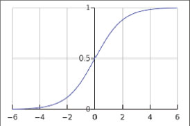
Figure. 5. Sigmoid Function
7.2.2. Hyperbolic Tangent Function
Another sort of activation function is the hyperbolic tangent (tanh) function. The hyperbolic tangent function is a nonlinear S-shaped function. Where the key distinction is that the tanh function's output range is zero-centered [-1, 1] rather than [0, 1], as illustrated in Figure 6 (Chigozie et al., 2018). As a result, in training, the hyperbolic tangent function is favored, as shown in Equation 10:
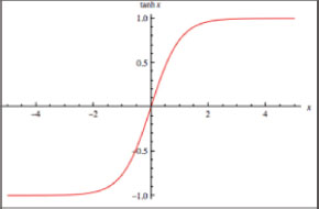
Figure. 6. Tanh Function
7.2.3. Rectified Linear Unit Function
Rectified Linear Unit (ReLU) functions, as defined mathematically in Equation 11, compress the net input to a value greater or equal to zero by setting the negative input values to zero; this is depicted in Figure 7. ReLU calculations were less expensive than sigmoid and tanh function computations since there is no calculation of the exponential function in activations, and sparsity may be used. The benefits of utilizing ReLU in neural networks include quick and efficient convergence and no gradient diminishing (Chigozie et al., 2018).
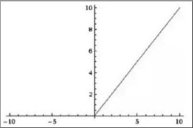
Figure. 7. ReLU Function
7.2.4. SoftMax Function
The SoftMax function is a function that is occasionally used in the output layer of NNs for classifications and is technically stated as demonstrated in Equation 12. The SoftMax function is a more extended logistic activation function that is used for multi-class classifications (Chigozie et al., 2018).
7.3. Training
The neural network is trained using a training set that uses supervised learning to discover network parameters with the lowest error rate. The method generates a function that associates a given input with a class label; Where the goal denotes that the learning function may be utilized for previously unknown mapping inputs, which necessitates the function to model the underlying connection in the labeled samples from the training dataset (Sherry et al., 2018).
7.4. Loss Function
The capacity of machine learning prediction or statistical models is dependent on a loss function known as the cost or objective function. The core principle behind the loss function is to calculate the error rate between anticipated and correct target values. As a result, minimizing the output of the losing function yields the best-performing machine learning model; nevertheless, there are numerous types of loss functions (Safwan and Yaser, 2013). Furthermore, these loss functions are used in conjunction with certain activation functions as indicated in Equation 13. The mean squared error (MSE) is a loss function that is used to calculate the average squared difference between actual and predicted target data.
Where N is the number of training samples, y^i is the model prediction value, and yi is the actual anticipated output. With hyperbolic tangent and linear activation functions, the Mean Squared Error (MSE) is commonly utilized. Moreover, it is presumptuous that the errors are regularly distributed.
7.5. Learning Rate
The learning rate is a measure of fit that specifies how much the model should change due to the predicted error each time the model weights are updated. Essentially, the researchers must decide where to step before determining the most recent direction at each advancement of traveling vertically to the curve. If the authors set a shallow learning rate, the training process may take a long time (Nikhil, 2017). However, if the researchers set a learning rate that is too high, then it would most likely begin to drift away from the minimum, as illustrated in Figure 8.
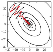
Figure. 8. Learning Rate at a Different Rate
8. Evaluation Metrics Methods
After developing a model, one of the most crucial phases is to evaluate its training and forecasting performance. Claims of the success of multi-layer algorithms frequently characterize the algorithm's quality using an essential set of performance measures (Guy et al., 2019).
8.1. Accuracy
An algorithm might be evaluated using test data, with predictions from testing separated into four sets. In terms of categorization, the True Positives (TP) data was positive; it is also anticipated to be positive, whereas the True Negatives (TN) data was negative and is predicted to be negative. The data of False Positives (FP) was negative but was predicted to be positive. The data of False Negatives (FN) was positive yet forecasted to be negative, as indicated in Equation 14. A classification accuracy rate is calculated by dividing correct predictions by the total number of produced predictions (Georgios et al., 2019) (Sherry et al., 2018).
8.2. Precision/Recall
To assess the algorithm's efficacy, two metrics (precision and recall) were used. As illustrated in Equations 15 and 16, recall (R) is a measure of the rate of documents effectively described by the algorithm, whereas precision (P) is a measure of the percentage of returned documents that were true (Arvinder et al., 2019).
8.3. F1-Score
A system with a high recall but low accuracy produces large outcomes. Nonetheless, when compared to the training labels, the majority of its predicted labels would be inaccurate. Systems with great accuracy but low recall provide few results, but the overwhelming majority of their forecasted labels are accurate when compared to training labels. When determining how well a system operates, it may be useful to have a single number to define the performance (Mohammed, 2021). This may be accomplished by calculating the combined metric F1-score associated with the method as the harmonic mean of the recall and precision ratios, as stated in Equation 17. The F1-score may be regarded as the average of the two, considering how comparable the two results were (7).
9. Methodology
This section discusses the architectural design for utilizing a deep learning model (LSTM) to categorize Twitter sentiment analysis. These deep networks are trained using a set of tweets, where the models are assessed using evaluation metrics. This paper's approach is separated into two sections. First, a diagram to show a simple description of the functioning mechanism; second, model development describing how to build deep learning models with their algorithms and mathematical foundations.
9.1. Twitter Sentiment Analysis Classification Steps
This work is completed in five stages. The first stage involves acquiring the dataset and then preprocessing it and using word embedding to represent the text and split it, using the outlier approach. Later, the LSTM model was developed, and ultimately, multiple metrics such as (accuracy, recall, and precision) are used to evaluate model performance, as shown in Figure 9 (Halina and Mohammed, 2017).
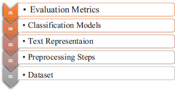
Figure. 9. Classification Steps of Twitter Sentiment Analysis
9.1.1. Dataset
The dataset for this paper (Twitter sentiment analysis.CSV file) was obtained from kaggel.com. This dataset contains around 1,600,000 records gathered through Twitter API streaming, and their features are shown as follows (target, ids, flag, user, text). The dataset was separated into 800,000 positive tweets and 800,000 negative tweets after the missing rows were removed. The dataset is read by the pseudocode in Algorithm 1.
Algorithm 1: Read Dataset and Removing the Missing Row |
Input: All tweets dataset (CSV-File) |
9.1.2. Preprocessing Steps
The content in this section was first modified by eliminating (stopwords, punctuation, lower case letters, white spaces, and special characters.
Stage (1) Stopword removal: Stopwords are meaningless words in a language that generate distortion when considered as text classification data. These terms are frequently used in sentences to effectively link ideas or assist with sentence structure. Prepositions, conjunctions, and some pronouns, such as {that, this, too, was, what, when, where, who, and would, are all called stop words}.
Stage (2) Punctuation removal: Punctuation that does not have many variants of the same word is eliminated. If these punctuations are not eliminated, data should be considered as {been, been@ been!} Separately as distinct terms {! @, [/], and?} are some punctuation examples.
Stage (3) Lower case and white space removal: Lowercasing is eliminated from all of our text data, which is one of the simplest and most successful ways of text preparation. It is applicable to the majority of text categorization and NLP issues with predicted output consistency. Furthermore, joining and splitting functions have been used to eliminate all white spaces in a string.
Stage (4) Special character removal: Finally, non-alphabetic or numeric special characters such as {$, %, &…. etc.} should be eliminated from all text as shown in Figure 10, that depicts the steps of text cleaning.
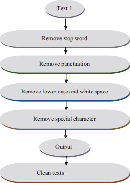
Figure. 10. Stages of Texts Cleaning
Stemming, a preprocessing step utilized in most text categorization algorithms, is also provided. Stemming returns words to their original form (root), reducing the number of word forms or classes in the data. Running, Ran, and Runner, for example, will be reduced to the word run.
9.1.3. Text Representation Step
In this section, the text representation procedures, carried out as part of preprocessing, involved the following stages:
Stage (1): Prior to text representation, the dataset was fragmented using the holdout technique, with the dataset divided into two partitions. The training set receives 80% of the data, whereas the testing set receives 20%.
Stage (2): Every word frequency inside the dataset was collected to identify (N) main common words (after trial results, the researchers identified the most common words that offer the best result equals 6000), and each of these words was assigned a unique integer ID. For example, ID0 is assigned to the most major common word, ID1 to the next significant word, and so on. Then, replace each common term with its assigned ID and delete any single words. It should be noted that the 6000 most common terms barely cover the majority of the content. As a result, the cleaned text loses some information.
Stage (3): The LSTM units require a fixed length input vector. More than 300 words have been omitted. The original text string was converted to a fixed-length integer vector while the word order was preserved. Finally, a word embedding is used to move each word indicated by its ID to a 32-dimensional vector. Every word is represented as a vector based on word concurrences using word embedding. When two words appear often in the text, they are more similar, and the distance between the respective vectors is short. Furthermore, text representation is regarded as a critical stage since it involves converting every tweet in raw text to fixed-size vectors, as shown in detail in Algorithm 2.
Stage (4): An embedding layer is a word embedding developed in collaboration with a neural network model on a particular natural language processing activity, such as language modeling or document categorization.
Algorithm 2: Preprocessing Steps |
Input: a cleaned collection of labeled texts extracted from tweets dataset |
9.1.4. Keras in Python
Keras in Python provides an embedding layer for neural networks on text data. It requires the input data to be an encoded integer ID, such that each word is represented by a unique number. The embedding layer is seeded with random weights and learns embedding for all training datasets. It is a versatile layer that may be utilized in a variety of ways, including:
• It may be used on its own to learn a word embedding that can subsequently be stored and utilized in another model.
• It may be utilized as part of a deep learning model in which the model learns the embedding itself.
• As a sort of transfer learning, it may be used to load a pre-trained word embedding model.
The embedding layer, a deep learning model in which the model itself learns the embedding, was utilized by the researchers in this article. The first hidden layer of a network is designated as the embedding layer. Three parameters must be supplied in this layer:
• Input dim: This is the words in the text data's vocabulary. For example, if your data is integer encoded to values ranging from 0 to 10, the vocabulary size would be 11.
• Output dim: This is the dimension of the vector space in which the words are to be embedded. It specifies the length of the output vectors generated by this layer for each word. It might, for example, be 32, 100, or much more significant.
• Input length: This is the length of input sequences, as defined for every Keras model input layer. This would be 1000 if all of the input documents were of a length of 1000 words. An embedding layer with a vocabulary of 30 encoded words, a vector space of 32 dimensions in which words are to be embedded, and input documents (tweets) containing 30 words apiece are used.
9.1.5. Classification Steps
The purpose of this section is to demonstrate the most important aspect of the proposed model. It shows how to use DL models (LSTM) and creates neural networks to assist in accurately identifying tweets. The input dimensions were (train-x) samples, while the output dimensions (train-y) were binary outcomes (one for positive and one for negative). This model had dropout and sigmoid output layers as shown in Figure 11. A generic block diagram was used to summarize the proposed models (LSTM).
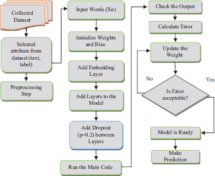
Figure. 11. The Main Diagram of The Proposed Models
9.2. Construction of the LSTM Model
To provide predictions, the proposed deep neural network model (LSTM model) was conceived and implemented. To accomplish so, the layers used to build the LSTM model were specified. One input layer, three hidden layers (embedding layer, convolutional layer, and LSTM layer), and one output layer comprise the deep neural network structure. The LSTM model is seen in Figure 12. In the structure of the LSTM model, tweet samples are trained and evaluated in the LSTM model.
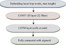
Figure. 12. The Proposed Model of LSTM
9.2.1. Training Phase
This section describes the first classification model, LSTM. The (train-x) data is fed into the model to train the LSTM; linked weights adjust until the error value between the goal (train) and the LSTM predicted value is minimized. Because the LSTM model is binary, the binary cross-entropy loss function was used to calculate the difference between the exact distribution (which the LSTM method is attempting to match) and the predicted distribution. The training phase of this network is divided into two parts: feed-forward and backpropagation. The LSTM model's feed-forward phase consists of two steps:
Step (1): The input layer in this step consists of train-x samples of a vocabulary set of 6k words supplied to the embedding layer. The embedding layer is the model's initial hidden layer. These words are represented as numbers contained in a vector of 32 dimensions. The embedding layer learns with the model. This layer converts words into a fixed-size vector and searches for similarity-related terms. To avoid overfitting, we added a dropout layer and adjusted the dropout probability to 0.5 during the training phase. The embedding layer's retrieved words are subsequently placed into the LSTM layer. This layer includes (100 cells), each with three gates.
Step (2): These three gates analyze the words to create a word sequence. They are then sent to a fully linked layer. Using a sigmoid function, the last dense layer turns the vector into a single output in the range of (0 or 1) The error is calculated using a binary cross-entropy loss function. Finally, during the backpropagation phase, we compute the difference between expected and goal output and then apply an Adam optimization technique to change the weight values.
9.2.2. Testing Phases
The evaluation function may be used to assess the trained model after creating the LSTM model and adapting it to the training dataset. This is an estimate based on unobserved data. The assessment is based on the correct prediction of the tested labels (test-y). The accuracy measure is used to assess the model's real-world performance. The LSTM model's training and testing procedures are described in Algorithm 3. The final LSTM model was built after selecting the best hyperparameter from those (LSTM cell (100), learning rate (0.1), batch size (64) fixed in the algorithm below based on the trial-and-error method, which is considered by varied attempts that are continuously repeated until success is achieved or until the practice stops trying.
Algorithm 3: Training and Testing Steps of LSTM Model |
Input: {X1, X2…… Xn} (samples of [text: integer numbers] records) Output: Classification results Required hyperparameter num of epoch =10, batch size =64, num cells of LSTM=100, Size of words 30 k, max length=300, Vector length=32, learning rate =0.001, β1=0.9, β2=0.999, η=10−8 Initialize Weights (W) = random number between (0,1) Initialize Bias =1 Define hidden layers: (Embedding layer, LSTM layer) For 1 to (number of epoch) do For 1 to (batch size) do Step 1: Create an embedding layer with 6 k input words, 32 vector length, and 500 max lengths of each sentence to represent each word as a vector. Step 2: LSTM layer: the output of the embedding layer inserted into the LSTM layer input. The bellow formulas are applied to compute the three gates (input, output, and forget gates), cell, and hidden state that generates a sequence of words. Step 3: The output of the LSTM layer pass through a fully connected layer with a sigmoid function to predict the final output results (0 or 1) Step 4: Calculate the error by using binary cross-entropy Step 5: Update weights by using (Adam optimization) End for End for Step 6: Calculate the final results using (Accuracy, Recall, Precision, and F1-score) as defined in equations (14) to (17). Step 7: Shows the results in the confusion matrix and history charts. END |
9.3. Experimental Results of the Proposed Model
The outcomes of the practical stages of the proposed model are discussed first, with an illustration of the Twitter dataset details and their contents after selecting only the text and label characteristics. Table 1 displays five entries before selecting only the text and label from the dataset and working on them.
Table 1. Five Records from the Dataset of Tweets
# |
Target |
IDS |
Date |
Flag |
User |
Text |
0 |
0 |
1467810369 |
Mon Apr 06 22:19:45 PDT 2009 |
no_query |
_TheSpecialOne_ |
@switchfoot http://twitpic.com/2y1zl-Awww,t… |
1 |
0 |
1467810672 |
Mon Apr 06 22:19:49 PDT 2009 |
no_query |
scotthamilton |
Is upset that he can’t update his Facebook by… |
2 |
0 |
1467810917 |
Mon Apr 06 22:19:53 PDT 2009 |
no_query |
mattycus |
@Keinichan I dived many times for the ball. Man… |
3 |
0 |
1467811184 |
Mon Apr 06 22:19:57 PDT 2009 |
no_query |
ElleCTF |
My whole body feels itchy and like it’s on fire |
4 |
0 |
1467811193 |
Mon Apr 06 22:19:57 PDT 2009 |
no_query |
Karoli |
@nationwideclass no, it’s not behaving at all… |
There was no need for a balancing step because the dataset was relatively balanced. Figure 13 shows each tweet segment in its original text and its new text after preprocessing processes. Preprocessing comprises removing stop words, punctuation, white space, and non-characters from the text to achieve a better representation when utilizing a word embedding layer to obtain an understanding of the text. In addition, all letters are uniform to be small letters. The data must be cleaned to improve word representation; Otherwise, the common words would be learned; and the keywords would have been disregarded, lowering classification accuracy.
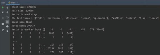
Figure. 13. Text Before and After Preprocessing Steps
As input for the proposed model, the dataset had been divided into two parts (20% for testing and 80% for training). The frequency of words in all texts is estimated to illustrate which words are the most influential in the texts and which are the least important, as shown in Figure 14.
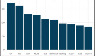
Figure. 14. Words Associated with Positivity
Each word is allocated a unique ID based on its frequency. For example, because the word 'said' has the highest frequency, it is allocated to ID0, and the word with the next highest frequency is assigned to ID1, and so on. The ID of the terms in texts is shown in Figure 15.
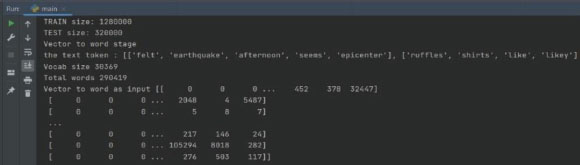
Figure. 15. ID Number of Each Word
Furthermore, because the proposed model demands a fixed-size entry, the researchers needed to know how many words we would utilize and the maximum length of the input phrases. As Figure 16 depicts the model diagram, which illustrates the proposed model in detail.
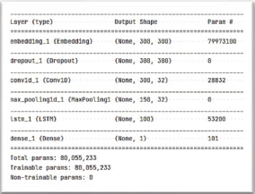
Figure. 16. The Proposed Model
Table 2 shows the optimum hyperparameter that yields the highest accuracy result (93.91%) in the proposed model.
Table 2. The Hyperparameters of the Proposed Model
Hyperparameter |
Choice |
Split dataset |
80% train 20% test |
Max length |
300 max lengths |
LSTM units |
100 units |
Dropout |
0.2 |
Batch size |
64 |
Num of Epochs |
10 epochs |
Learning rate |
0.001 |
The hyperparameter values that the researchers selected are the most acceptable for the dataset. Figures 17, 18, and 19, respectively, depict the model's accuracy and the loss model in the proposed model.
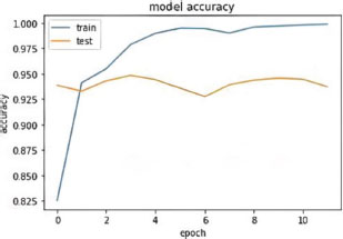
Figure. 17. Accuracy Result of LSTM Model
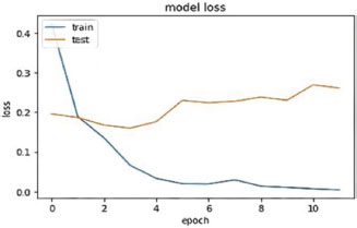
Figure. 18. Loss Result of LSTM Model
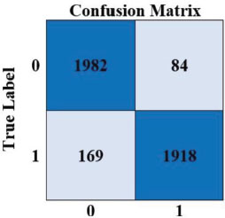
Figure. 19. Confusion matrix of proposed model
The confusion matrix contrasts the classification model's correct and erroneous predictions with the actual results (the target value). The classification results revealed that the recommended classifier had an accuracy of 93.91 percent. A confusion matrix containing TP, TN, FP, and FN values produced Figure 19.
10. Conclusions
In conclusion, the method's findings were extracted from the experiment results of the proposed technique as follows: First, a technique has been proposed for gathering, filtering, analyzing, and interpreting Twitter data using sentiment analysis; Second, in this study, more than 1,600,000 tweets were used to develop a functional and attempted method. By gathering tweets over a long period or using the Twitter Search API more often, the volume of data may rise; Additionally, machine learning methods, such as CNN and LSTM have the highest accuracy. The hybrid model (CNN-LSTM classifier) was used to construct the model, which had the highest accuracy. The overall accuracy rating was 93.91%; Furthermore, the preprocessing step is crucial since it has a significant impact on the classification's accuracy. When applying the proposed technique to this dataset, Adam's optimization strategy improved classification accuracy significantly. Generally, this research examines and compares current opinion mining methodologies, such as machine learning, text mining, and assessment criteria.
11. References
Abdullah, A., and Faisal, S. 2017. Data privacy model for social media platforms. In 2017 6th ICT International Student Project Conference (ICT-ISPC) (pp. 1–5). IEEE.
Abdullah, A., and Mohammed, H. 2019. Social Network Privacy Models. Cihan University-Erbil Scientific Journal, 3(2), 92–101.
Ajay, Sh., and Ausif, M. 2019. Review of deep learning algorithms and architectures. IEEE access, 7, 53040–53065.
Alexander, V. 2019. LSTM networks for detection and classification of anomalies in raw sensor data (Doctoral dissertation, Nova Southeastern University).
Ali, N., Elnagar, A., Shahin, I., and Henno, S. 2021. Deep learning for Arabic subjective sentiment analysis: Challenges and research opportunities. Applied Soft Computing, 98, 106836.
Andreas, S., and Faulkner, Ch. 2017. NLP: the new technology of achievement, NLP Comprehensive (Organization), New York, Morrow.
Arvinder, B., Mexson, F., Choubey, S., and Goel, M. 2019. Comparative performance of machine learning algorithms for fake news detection. In International conference on advances in computing and data sciences (pp. 420–430). Springer, Singapore.
Asil, C., Dilek, H., and Junlan, F. 2010. Probabilistic model-based sentiment analysis of twitter messages. In 2010 IEEE Spoken Language Technology Workshop (pp. 79–84). IEEE.
Balakrishnan, G., Priyanthan, P., Ragavan, T., Prasath, N., and Perera, A. 2012. Opinion mining and sentiment analysis on a twitter data stream. In International conference on advances in ICT for emerging regions (ICTer2012) (pp. 182–188). IEEE.
Chigozie, N., Ijomah, W., Gachagan, A., and Marshall, S. 2018. Activation functions: Comparison of trends in practice and research for deep learning. arXiv preprint arXiv:1811.03378.
Christopher, C. 2020. Improving t-SNE for applications on word embedding data in text mining.
Deborah, W., Ardoin, N., and Gould, R. 2021. Using social network analysis to explore and expand our understanding of a robust environmental learning landscape. Environmental Education Research, 27(9), 1263–1283.
Fahad, M., Ahmed, A., and Abdulbasit, S. 2020. Smiling and non-smiling emotion recognition based on lower-half face using deep-learning as convolutional neural network. In Proceedings of the 1st International Multi-Disciplinary Conference Theme: Sustainable Development and Smart Planning, IMDC-SDSP 2020, Cyperspace, 28–30 June 2020.
Geetika, G., and Yadav, D. 2014. Sentiment analysis of twitter data using machine learning approaches and semantic analysis. In 2014 Seventh international conference on contemporary computing (IC3) (pp. 437–442). IEEE.
Georgios, G., Vakali, A., Diamantaras, K., and Karadais, P. 2019. Behind the cues: A benchmarking study for fake news detection. Expert Systems with Applications, 128, 201–213.
Govindarajan, M. 2021. Educational Data Mining Techniques and Applications. In Advancing the Power of Learning Analytics and Big Data in Education (pp. 234–251). IGI Global.
Guy, H., Kok, H., Chandra, R., Razavi, A., Huang, S., Brooks, M., and Asadi, H. 2019. Peering into the black box of artificial intelligence: evaluation metrics of machine learning methods. American Journal of Roentgenology, 212(1), 38–43.
Halina, I., and Mohammed, H. 2017. A Review of Blended Methodologies Implementation in Information Systems Development Abdullah AbdulAbbas Nahi1. Muhammad Anas Gulumbe2. Nurul Syazana Selamat3. Noor Baidura.
Jan, L., Mohammadi, M., Mohammed, A., Karim, S., Rashidi, S., Rahmani, A., and Hosseinzadeh, M. 2021. A survey of deep learning techniques for misuse-based intrusion detection systems.
Jasim, Y, and Mustafa, S. 2018. Developing a software for diagnosing heart disease via data mining techniques.
Juan, C. 2021. Efficient Digital Management in Smart Cities.
Judith, B., Michael, B., Danica, K., and Kjellstrom, H. 2017. Deep representation learning for human motion prediction and classification. In Proceedings of the IEEE conference on computer vision and pattern recognition (pp. 6158–6166).
Manuel, R., Gütl, C., and Pietroszek, K. 2021. Real-time gesture animation generation from speech for virtual human interaction. In Extended Abstracts of the 2021 CHI Conference on Human Factors in Computing Systems (pp. 1–4).
Marina, P., and Emanuele, F. 2020. Multidisciplinary pattern recognition applications: a review. Computer Science Review, 37, 100276.
Matthew, C., Castelfranco, A., Roncalli, V., Lenz, P, and Hartline, D. 2020. t-Distributed Stochastic Neighbor Embedding (t-SNE): A tool for eco-physiological transcriptomic analysis. Marine genomics, 51, 100723.
Mohammed, Sh. 2019. Design a Mobile Medication Dispenser based on IoT Technology. International Journal of Innovation, Creativity and Change, 6(2), 242–250.
Mohammed, Sh. 2021. Improving Coronavirus Disease Tracking in Malaysian Health System. Cihan University-Erbil Scientific Journal, 5(1), 11–19.
Mohammed, T., and Jose, C. 2020. Embeddings in natural language processing: Theory and advances in vector representations of meaning. Synthesis Lectures on Human Language Technologies, 13(4), 1–175.
Muhamad, A., Yaser, J., Mostafa, W., Mustafa S., and Sadeeer A. 2021. High-Performance Deep learning to Detection and Tracking Tomato Plant Leaf Predict Disease and Expert Systems.
Mustafa, A., Yaser, J., Tawfeeq, F., and Mustafa, S. 2021. On Announcement for University Whiteboard Using Mobile Application. CSRID (Computer Science Research and Its Development Journal), 12(1), 64–79.
Nasim, R., Baratin, A., Arpit, D., Draxler, F., Lin, M., Hamprecht, F., and Courville, A. 2019. On the spectral bias of neural networks. In International Conference on Machine Learning (pp. 5301–5310). PMLR.
Neethu, S., and Rajasree, R. 2013. Sentiment analysis in twitter using machine learning techniques. In 2013 fourth international conference on computing, communications and networking technologies (ICCCNT) (pp. 1–5). IEEE.
Neha, K., and Bhilare, P. 2015. An Approach for Sentiment analysis on social networking sites. In 2015 International Conference on Computing Communication Control and Automation (pp. 390–395). IEEE.
Nik, H., Prester, J., and Wagner, G. 2020. Seeking Out Clear and Unique Information Systems Concepts: A Natural Language Processing Approach. In ECIS.
Nikhil, B. 2017. Fundamentals of Deep Learning: Designing Next-generation Artificial Intelligence Algorithms/c Nikhil Buduma. Beijing, Boston, Farnham, Sebastopol, Tokyo: OReilly.
Niloufar, Sh., Shoeibi, N., Hernández, G., Chamoso, P., and Juan, C. 2021. AI-Crime Hunter: An AI Mixture of Experts for Crime Discovery on Twitter. Electronics, 10(24), 3081.
Peng, Ch., Sun, Z., Lidong B., and Wei, Y. 2017. Recurrent attention network on memory for aspect sentiment analysis. In Proceedings of the 2017 conference on empirical methods in natural language processing (pp. 452–461).
Priyanka, D., and Silakari, S. 2021. Deep learning algorithms for cybersecurity applications: A technological and status review. Computer Science Review, 39, 100317.
Rohit, K. 2018. Fake news detection using a deep neural network. In 2018 4th International Conference on Computing Communication and Automation (ICCCA) (pp. 1–7). IEEE.
Safwan, H., and Yaser, J. 2013. Diagnosis Windows Problems Based on Hybrid Intelligence Systems. Journal of Engineering Science & Technology (JESTEC), 8(5), 566–578.
Sagar, B., Doshi, A., Doshi, U., and Narvekar, M. 2014. A review of techniques for sentiment analysis of twitter data. In 2014 International conference on issues and challenges in intelligent computing techniques (ICICT) (pp. 583–591). IEEE.
Seyed-Ali, B., and Andreas, D. 2013. Sentiment analysis using sentiment features. In 2013 IEEE/WIC/ACM International Joint Conferences on Web Intelligence (WI) and Intelligent Agent Technologies (IAT) (Vol. 3, pp. 26–29). IEEE.
Sherry, G., Amer, E., and Gadallah, M. 2018. Deep learning algorithms for detecting fake news in online text. In 2018 13th international conference on computer engineering and systems (ICCES) (pp. 93–97). IEEE.
Thabit, Th., and Jasim, Y. 2017. Applying IT in Accounting, Environment and Computer Science Studies. Scholars' Press.
Thabit, Th., and Yaser, J. 2015. A manuscript of knowledge representation. International Journal of Human Resource & Industrial Research, 4(4), 10–21.
Thabit, Th., and Yaser, J. 2017. The role of social networks in increasing the activity of E-learning. In Social Media Shaping e-Publishing and Academia (pp. 35–45). Springer, Cham.
Xipeng, Q., Sun, T., Xu, Y., Shao, Y., Dai, N., and Huang, X. 2020. Pre-trained models for natural language processing: A survey. Science China Technological Sciences, 63(10), 1872–1897.
Yaser, J. 2018. Improving intrusion detection systems using artificial neural networks. ADCAIJ: Advances in Distributed Computing and Artificial Intelligence Journal, 7(1), 49–65.
Yaser, J., Mustafa, O., and Mustafa, S. 2021. Designing and implementation of a security system via UML: smart doors. CSRID (Computer Science Research and Its Development Journal), 12(1), 01–22.