
Regular Issue, Vol. 11 N. 1 (2022), 111-128
eISSN: 2255-2863
DOI: https://doi.org/10.14201/adcaij.28093
|
ADCAIJ: Advances in Distributed Computing and Artificial Intelligence Journal
Regular Issue, Vol. 11 N. 1 (2022), 111-128 eISSN: 2255-2863 DOI: https://doi.org/10.14201/adcaij.28093 |
A Hybrid System For Pandemic Evolution Prediction
Lilia Muñoza,b, María Alonso-Garcíac, Villarreal Vladimira,b, Guillermo Hernándezd, Mel Nielsena, Francisco Pinto-Santosd, Amilkar Saavedraa, Mariana Areizaa, Juan Montenegroa, Inés Sittón-Candanedob, Yen Caballero-Gonzálezb, Saber Trabelsie, and Juan M. Corchadoc, d, f, g
a Grupo de Investigación en Tecnologías Computacionales Emergentes (GITCE), Universidad Tecnológica de Panamá, Panamá
b Centro de Estudios Multidisciplinarios en Ciencia, Ingeniería y Tecnología (CEMCIT-AIP), 0819 Panama City, Panama
c Air Institute, Salamanca, Spain
d BISITE Research Group, University of Salamanca. Calle Espejo s/n. Edificio Multiusos I+D+i, 37007, Salamanca, Spain
e Texas A&M University at Qatar, Qatar
f Department of Electronics, Information and Communication, Faculty of Engineering, Osaka Institute of Technology, Osaka, Japan
g Pusat Komputeran dan Informatik, Universiti Malaysia Kelantan, Kelantan, Malaysia
ABSTRACT
The areas of data science and data engineering have experienced strong advances in recent years. This has had a particular impact on areas such as healthcare, where, as a result of the pandemic caused by the COVID-19 virus, technological development has accelerated. This has led to a need to produce solutions that enable the collection, integration and efficient use of information for decision making scenarios. This is evidenced by the proliferation of monitoring, data collection, analysis, and prediction systems aimed at controlling the pandemic. To go beyond current epidemic prediction possibilities, this article proposes a hybrid model that combines the dynamics of epidemiological processes with the predictive capabilities of artificial neural networks. In addition, the system allows for the introduction of additional information through an expert system, thus allowing the incorporation of additional hypotheses on the adoption of containment measures.
KEYWORD
COVID-19; SIR model; compartmental models; long short-term memory; prediction
1. Introduction
Many countries have already rolled out their vaccination programs and are progressing steadily, however, many others experience severe vaccine shortages, all the while new, possibly vaccine-resistant variants of COVID-19 emerge. It is therefore essential to continue taking measures that will help curb the spread of the virus and its variants. One of the impediments to the optimal management of the pandemic is the lack of reliable statistics on the morbidity and mortality rate, as well as other related factors. At the beginning of the pandemic, many decisions were taken by trial and error, as there was a lack of information on the new severe acute respiratory syndrome coronavirus 2 (SARS-CoV-2).
Had governments understood the risk of a global health crisis when the first cases had been detected in China in January 2020, they would have been able to establish stricter measures since the very beginning. Unfortunately, this has not been so, and COVID-19 spread rapidly in February 2020 throughout Asia and Europe. Since then, cases have been detected across all continents. It is estimated that up until now, there have been over 225 million cases worldwide, among which 4.6 million were mortal, although these statistics increase daily.
Had intelligent systems for data collection and pandemic monitoring been implemented since the start of the pandemic, these figures would have been much lower today and the build-up to critical situations, such as the lack of face masks and ventilators, the overflow of hospitals, virus waves, and the closing down of all businesses, could have been prevented. Access to contagion estimates would have meant that governments could have planned for the production and purchase of medical equipment, avoiding both equipment shortage and overspending. Predictions of COVID-19 rates would have enabled hospitals to cater for an increased number of admissions; prepare extra beds in intensive care units and set up temporary healthcare support facilities ahead of time, transporting resources from localities in which COVID rates were low to those in which they were high. All this means that information and technology are the keys to increasing the efficiency of our healthcare systems, preventing future waves, and combating the pandemic.
These examples serve to show that it is necessary to develop technologies and systems capable of predicting the near-future and far-future evolution of this pandemic and the emergence of future pandemics. It is also necessary to be able to assess the impact that different measures, such as lockdown, confinement, the closing of businesses, curfew, etc., have on the spread rate. Artificial intelligence (AI) can provide us with this ability, specifically, explainable artificial intelligence (XAI), whose reasoning processes are visible to humans, making it possible to understand how a system arrived at a specific conclusion.
Epidemiological prediction is a branch of epidemiology in which there has been renewed interest following the abrupt emergence of COVID-19. An overview of the state of the art from different perspectives may include sociophysics (Tanimoto, 2021), biomathematics (Mondaini, 2020), and artificial intelligence (Le Gruenwald and Jain, 2021). State-of-the-art literature identifies game theory (Bauch, 2005) and evolutionary game theory methods (Kabir and Tanimoto, 2019; Kabir and Tanimoto, 2020) as noteworthy approaches on prediction. The formal framework introduced in these works makes it possible to evaluate the costs of imposing restrictive measures in terms of economic and epidemiological impact.
The motivation behind this proposal lies in achieving the ability to monitor and predict the evolution of coronavirus in Panama. The Panamanian Ministry of Health confirmed a total of 365,104 total cases of COVID-19 in Panama, from the start of the pandemic until May 2, 2021. As for 2020, Panama experienced the highest number of COVID-19 cases per 100,000 inhabitants in Latin America, which has had a strong impact on its GDP (Gross domestic product), in an economy that relies heavily on air transportation, tourism, and construction. According to the statistics, Panama is currently one of the worst-hit countries in Central America, in addition to the high spread rate, poverty has increased by two percentage points, while public debt shot up by almost 20 percentage points of GDP. Panama must now overcome the challenge of reviving its economy and mitigating poverty while combating the pandemic.
The developed system is capable of aiding the Panamanian government and doctors to take optimal decisions when managing the pandemic. Data analyses and predictions make it possible to distribute scarce medical resources to the regions in which they are most needed i.e., the ones in which the level of contagion is the greatest. Moreover, the system can help the local authorities select the most effective restrictive measures and loosen the restrictions in areas where the spread rate is low, this would also support the country’s economic recovery.
In epidemiological prediction systems, one of the most important advances in artificial intelligence is used, namely, the machine learning (ML) paradigm. ML neural nets can associate symbols with vectorized representations of data. This gives them the ability to understand what the data represents. ML models are capable of creating new rules and modifying /discarding the old ones. This is unlike symbolic reasoning, where the system does not comprehend the meaning behind the symbols. Thus, since the beginning of the pandemic, many machine learning models have been employed as support tools, especially to foresee future spread levels. For a detailed revision of paradigms in COVID prediction, the reader can refer to (Perc et al., 2020; Yousaf et al., 2020; Bertozzi et al., 2020).
Deep learning, a subset of machine learning, has been used in numerous proposals. For example, a deep convolutional neural network has been adapted for the classification of chest X-ray images of COVID-19 patients (Ozturk et al., 2020). In (Chimmula and Zhang, 2020) the authors have used deep learning-based LSTM (Long short-term memory) networks to predict the transmission of COVID in Canada. However, the use of a single AI approach normally implies some limitations, so in order to achieve optimal and highly accurate results, it is recommendable to combine two or more AI-based methods. An example of this approach are the deep neuro-fuzzy algorithms that are implemented in smart systems employing techniques based on fuzzy logic and deep neural networks. The optimal performance of this approach has been demonstrated in practice in (Castillo Ossa et al., 2021), where the authors have used a combination of mathematical modeling and recurrent neural networks to predict COVID-19 evolution in Colombia.
Panamanian medical authorities are currently using the developed model to curb the pandemic. This project has been conducted under the EPIDEMPREDICT for COVID-19, code GCHF5076720. It has been sponsored by the Panamanian Secretaría Nacional de Ciencia Tecnología e Innovación (SENACYT).
This article is organized as follows: Firstly, in section 2, the proposed system is presented and its use case is described. In section 3 the proposed system is evaluated with the available data, giving a quantitative measure of its predictive capability. Lastly, section 3 draws conclusions from the conducted study.
2. Proposal and use case: Panama COVID-19 prediction
The developed system is based on a hybrid model incorporating SIR model population dynamics, as well as LSTM recurrent neural networks. It has been designed to forecast the transmission rate of the virus in Panama. This hybrid solution, combining an expert system and LSTM in the SIR model, provides explainable results, evidencing the impact of restrictive measures on the fluctuation of the coefficient. Moreover, expert rules help predict the effect of the implementation of such measures on the spread rate. The system implements explainable artificial intelligence which, in this case, helps understand the system’s interpretation of pandemic-related data, making it possible to modify the inputs or adjust the factors being monitored and predicted. Figure 1 shows the proposed solution whose characteristics are discussed in detail in the sections that follow.
Figure 1. Hybrid system overview
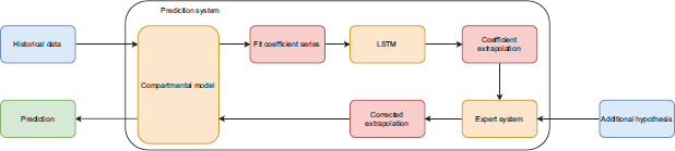
The evolution of the virus, in a given time period, is measured using a historical dataset and the curves S (the time-dependent susceptible population), I (the time-dependent infected population), and R (the time-dependent removed (recovered, death) population) are extracted for the established time period. These variables are used to fit an SIR model using sliding windows. The Runge-Kutta method is applied to solve the differential equations and the fit is performed in the sense of the least squares, which makes it possible to obtain the SIR model’s unknown parameters: β and γ, and the basic reproductive number R0, all those are functions of time. To extrapolate these parameters to higher time values, an LSTM neural network is used, the results of which are further refined by using an expert system that takes into account possible future changes in the constraints imposed by the government. Lastly, the forecast of the evolution of the S, I, R0 curves is made when the SIR model is solved together with the extrapolated coefficients.
The system was implemented in Python 3 using numpy 1.21, pandas 1.1.4, scipy 1.7.1, and tensorflow 2.6.1.
2.1. Input variable extraction
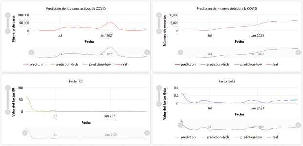
The Deep Intelligence platform (Corchado et al., 2021) has been used as the storage engine and central axis for the processing and management of data streams. This platform has been programmed to periodically ingest data on the evolution of COVID-19 in Panama (specifically, the data on the daily evolution of the population, active COVID cases, cumulative number of deaths, and cumulative number of recoveries), taken from the reports published by the Panamanian government on the official Ministry of Health website (Presentaciones Covid-19 - Ministerio de Salud, Gobierno de Panamá,). Thus, further on in this paper, this model is applied to keep the predictions updated (Figure 2).
Figure 2. Example of a prediction plotted on a Deep Intelligence dashboard
2.2. Compartment models
The initial development of the mathematical modeling of infectious diseases is owed to public health physicians. Daniel Bernouilli, who came from a renowned family of mathematicians, is the first one to have introduced and resolved a mathematical model for smallpox in the 18th century. Ever since then, the emerging and reemerging diseases shed light on the importance of the mathematical modeling of infectious diseases and revive a strong interest in the subject among scientists from different fields. Today, mathematical models play an important role in the authorities’ decision-making process. They provide important insights on the disease dynamic and can serve for testing and evaluating potential control strategies and as predictors of future outbreaks. Most importantly, models continue to mature with the ongoing advances in computational tools, access to the disease incidence data, and their combination with advanced mathematical and artificial intelligence-based algorithms.
The simplest mathematical models of infectious diseases are based on the idea of compartmental modeling. Indeed, the population under study is divided into compartments and the transmission of the disease from one compartment to another is described mathematically under meaningful assumptions on the nature and the time rate of the transfer. These compartmental models are often labeled in the literature as MSEIR, MSEIRS, SEIR, SEIRS, SIR, SEI, SEIS, etc., where each letter corresponds to a compartment of the population. For instance, S(t) denotes the number of individuals who are susceptible to the disease at time t (that is not yet infected or immunized at time t) whereas I(t) denotes the number of infected individuals who are able to spread the disease through contact with susceptible subjects, and R(t) denotes the number of individuals who have been infected and then excluded, assuming that they are not at danger of getting reinfected and spreading the disease. These models are basically systems of coupled first-order differential equations describing the evolution of the disease, and the threshold of these models is the famous basic reproduction number defined as the average number of secondary infections produced when one infected individual is introduced into a host population where everyone is susceptible. Other mathematical indicators such as contact number and replacement number can be defined and play a major role in the understanding and prediction of the disease dynamic. These models can be improved and extended very easily from the mathematical point of view.
The basic mathematical expression of compartmental models describing the dynamic of communicable diseases goes back to the works of W.O. Kermack and A.G. McKendrick published in 1927, 1932, and 1933, interested readers are referred to (Kermack and McKendrick, 1927; Kermack and McKendrick, 1932; Kermack and McKendrick, 1933). For instance, the simplest SIS model is based on the hypothesis that the size of the population N is assumed constant, that may be because the disease is not mortal or there is a balance between the death and birth rates. Also, the rate of new infections is given by mass action incidence (contact rate βN), individuals leave the infected compartment and return to the susceptible compartment at a rate aI per unit of time. The SIS model is given by
completed with initial data , and therefore . Observe that by summing up both differential equations we obtain , it is therefore assumed that the size of the population S +I = N for all time is propagated by the dynamic. In particular, one can replace N by N — 1 and observe that the system 1 can be recasted in a single differential equation reading
whose explicit solution is given by
It is rather easy to see from this equation that the infection declines, that is, the number of infections approaches zero, when β N / α < 1. In the contrary case, that is, when β N / α > 1, the infection persists. This explains why, in the literature, the particular constant solution I = 0 (corresponding to S = N) is called the disease-free equilibrium, and the constant solution I = N — α/β (corresponding to S = α/β) is called the endemic equilibrium. This also explains why the famous reproduction number is defined as R0 = βN/α and plays a crucial role in the prediction of the disease dynamic.
A slightly more complex model is the so-called SIR model, which is based on the same assumptions as presented above, except that the subject that has recovered from the infection is moved to a new «removed» compartment instead of going back to the «susceptible» compartment. The SIR model is given by
completed with initial data I0, S0, and R(t = 0) = R0. In particular, this model assumes a recovery rate of γI corresponding to a waiting time , that is the fraction that is still in the infected class t units after entering this compartment and to γ-1 as the mean waiting time. Again, by summing up the equations is obtained, that is, the total size of the population is constant. Therefore, the SIR system can be reduced to a system of two coupled differential equations. Indeed, dividing the equations by the total population size N, and denoting it by s = S / N, i = I/ N and r = R/N, we get
with r(t) = 1 — s(t) — i(t). The basic theory of differential equations shows that a unique solution (s(t), i(t)) of this system exists for all positive time on the set ; interested readers are referred to (Hethcote, 1976) for a detailed proof. In this model, the contact number is defined as , that is, the contact rate β per unit of time times the average infectious period γ-1. The initial (at t = 0) replacement number is . From the mathematical point of view, it can be shown that if (s(t), i(t)) is a solution of 3 in the set , then [see (Hethcote, 1976; Hethcote, 1989)]):
•If , then .
•If , then i(t) increases to a maximum value imax given by
•and then decreases to zero as .
•the susceptible fraction s(t) is a decreasing function and its limiting value s∞ is the unique root in (0,1 /σ) of the equation
In other words, the mathematical analysis of the SIR shows that it represents an epidemic outbreak very well. Indeed, in a typical epidemic outbreak, we see that the curve that represents the infected individual increases from an initial number I0 (close to 0), reaches a peak, and then decreases towards zero as a function of time. Also, the number of susceptible individuals always decreases to a certain final value (given above) and the epidemic declines when the number of peoples goes strictly below N/σ and the replacement number σS(t)/N goes below 1. The mathematical predictions are in correlation with the epidemic dynamic observations. A rather straightforward extension of this model allows to consider vital dynamics, that is, birth and death is given by
Observe that the total population is still conserved, as represented by . Therefore, dividing the above differential equations by the total population size (as it is conserved) leads to the following system
For this model, the reproduction number is defined as which is the contact rate P times the average death-adjusted infectious period 1/(γ+μ). From the mathematical point of view, the standard theory of differential equations allows to show that if σ ≤ 1 or I0 = 0, then the solution paths starting in approach the disease free equilibrium s = 1 and i = 0. However, if σ>1, then all the solution paths i0>0 approach the endemic equilibrium given by a susceptible fraction of 1/σ and an infected fraction of μ(σ − 1)/β. One of the major advantages of compartmental models resides in their flexibility in terms of mathematical modeling. Indeed, several compartments can be easily added so as to meet the particular properties of a population or a disease. Also, compartmental models can be solved on any basic computer, that is, there is no need for advanced numerical algorithms and/or computational power. Eventually, these models can be easily extended to take into account several properties of the population under study in the modeling phase, such as birth and non-disease related death rates, the age structure of the population, etc., as well other action mechanisms, such as temporary immunity, medical therapies, vaccination, and restrictions, such as social distancing, quarantine requirement, travel restrictions, etc. For instance, to take into account the loss of immunity, one might add a term θR to the susceptible equation and add the opposite term to the removed equation in the SIR model. Also, therapies (g) and vaccination (f) can be very easily modeled through integral delay terms of the following form
added from the infected equation and subtracted from the susceptible equations in an SIR model. In the above expression, θ denotes the disease transmission coefficient and individuals leave the susceptible compartment at a rate given by the integral , and h represents the maximum time taken to become infectious. Although compartmental models are very simple and provide a convenient modeling solution, they suffer from the gap of parameter estimation. They contain an important number of parameters whose values play a crucial role in the predictions and the forecasting of the disease dynamic and therefore have to be estimated very precisely. Thus, these parameters must be recovered from real-life data. The challenge to achieving this lies in connecting models and data; overcoming it has become crucial in the last decades. The most widely used method is the so-called Ordinary Least Square Estimation. Briefly, the idea is to link a statistical model to the process generated by the compartmental dynamical system at hand (SIS, SIR, SEIR, etc,) depending on a parameter θ (we consider only one parameter here for simplicity), assuming that the model output and associated random deviations (measurement error) are captured by the random variables
where z(tj, θ0) denotes the output of the mathematical model and the denote a set of random variables modeling the random deviations away from z(t, θ0) satisfying an adequate set of mathematical assumptions. Eventually, the quantity is minimized over a set of parameter vectors θ. Most techniques follow the same line, more precisely the Bayesian sequential data assimilation (or forecasting) approach based on Ensemble Kalman Filter, Markov Chain Monte Carlo, and the minimization of a functional cost over a set of admissible parameter vectors, and coupled to the deterministic or stochastic compartmental model dynamical model [(see (Engbert et al., 2021; Daza-Torres et al., 2021; Wang et al., 2020) and references therein]. A new research field in data assimilation for communicable diseases prediction and forecasting has become very attractive to scientists, with particular focus on COVID-19, namely the development of tools, techniques, and methods of data assimilation based on neural networks and artificial intelligence models, which is the aim of the present contribution. All the models of communicable diseases, presented and cited above, are based on ordinary differential or integro-differential equations since the involved quantities depend only on time. Introducing spatial dependence, in addition to time dependence, into the previous mathematical models, allows to model the geographical spread of a disease. Also, spatio-temporal dependence allows for the description of the migration of the susceptible population, such that the disease may be avoided, this can be achieved by introducing diffusive and chemotactic-like terms. Also, by opposition to the temporal models, the system parameters, such as the contact rate, can be a spatially dependent function of the distribution of infected people. To fix this idea, let’s consider the previously described SIR model and let β=β(t), that is, time-dependent. A simple, symmetric contact-term candidate, including a typical interaction radius, x0(t), can be written in the following Gaussian form [see (Kuperman and Wio, 1999)]
Therefore, normalizing the population size to 1, the space-time dependent SIR model now reads as follows
completed with the physically adequate set of boundary conditions and initial data. In the above system, ∇2 denotes the Laplacian, η models the diffusion coefficients whereas η models the chemotactic parameter. This system is composed of coupled nonlinear partial differential equations, and therefore its mathematical analysis and numerical simulations are much more demanding than the classical ordinary differential systems. Several related mathematical diffusive compartmental-based models were developed and analyzed in the literature, interested readers are referred to (Li et al., 2018; Suo and Li, 2020). Standard optimal control theories can be designed for this family of diffusive systems to fit the model with real-life data, and coefficient recovery processes can be rigorously designed, for more details readers are referred to any textbook on optimal control theory for PDEs [e.g., (Casas and Mateos, 2017; Tröltzsch, 2010)]. Recently, a novel technique of data assimilation has been developed in (Azouani et al., 2014) for a family of parabolic systems of partial differential equations in the two-dimensional Navier-Stokes equations and extended to several other systems, including the three-dimensional Tamed Navier-Stokes equation (Markowich et al., 2016). The idea is to introduce an interpolant operator and , modeling the real-time observations and measures, as a feedback controller into the original system given above, to obtain the following auxiliary system
completed with the same boundary conditions and zero initial data. Briefly speaking, the parameter h controls the size (or the amount of needed) observations and measurements and δ1 and δ2 are nudging parameters. What can be shown (for the models cited above) is that, for a class of interpolants operators , for sufficiently small h and sufficiently large δ1 and δ2, the solution of the latter system converges exponentially fast in time towards the original solutions. This means that the solutions of the original theoretical model are now nudged towards the observed and measured data. The linear interpolant operator can be chosen as the approximation of the identity, the projector onto the low Fourier modes, a nodal averaging operator etc. The combination of this novel data assimilation approach and the extrapolation method based on a neural network will be investigated in a forthcoming research work.
2.3. Extrapolation of the coefficients
Using the models introduced above, adjustments can be made by moving the windows of the coefficients that parametrize them, thus understanding them as functions of time. These parameters must be treated as time series whose extrapolation, using the equations that govern their dynamics, will allow to make predictions. In this case, due to the available data, an SIR model (2) has been considered, which makes it necessary to extrapolate the beta and gamma coefficients.
The series β(t) is extrapolated using a recurrent neural network called LSTM. (Abadi et al., 2015)
The series γ(t) is extrapolated by taking the median of the series γ(t) for t < tmax. This parameter does not fluctuate much as it is the inverse of the time it would take for a person to recover from the disease, therefore, it is a constant.
LSTM is a type of recurrent neural network able to efficiently solve tasks involving long time lags.
The fundamental component of this neural network is the memory block, in turn consisting of one or more memory cells and three gating units shared by them. Each memory cell is based on a core self-connected linear unit, the Constant Error Carousel (CEC), which provides short-term memory storage for long-term periods of time. The gates, called input, forget and output gates, are trained to control the information flow in the cell by learning the relevant information to store in memory, for how long it must be kept, and when to use it.
Let t = 0,1,2,... be discrete time steps, where all the units’ activations are updated at each time step (forward pass) and then error signals are calculated for all weights (backward pass).
In the following, denotes the vth memory cell of the jth memory block, is the weight on the connection from unit m to unit l, sc is the c cell state, and y is a gate activation; is the input to the cell and zin, zφ and zout are inputs to the input, forget and output gates. Let f be a logistic sigmoid function with range [0,1] and g a centered logistic sigmoid function with range [–2, 2].
At each forward pass, inputs and activations are computed as follows:
Thereby, when the input gate’s activation yin is close to 1, the relevant inputs are stored in the memory block. Then, the cell state is obtained according to:
In that way, when , the forget gate is opened and determines how long the information should be retained and when to remove it by resetting the cell state to zero.
Finally, the cell output yc is computed as:
To overcome back-flow error problems, LSTM backward pass is designed as a powerful combination of a slightly modified, truncated Back Propagation Through Time (BPTT) and a customized version of Real-Time Recurrent Learning (RTRL). BPTT is used in output units, while output gates employ a slightly modified, truncated version of BPTT. However, a shortened version of RTRL is used in weights to cells, input gates, and the new forget gates. Truncation indicates that once mistakes leak out of a memory cell or gate, they are cut off, however, they do serve to modify the incoming weights. As a result, the CECs are the only section of the system where errors can flow back indefinitely. This improves the efficiency of LSTM updates without sacrificing learning power: outside of cells, error flow tends to diminish exponentially.
The architecture used consisted of an LSTM with sigmoidal activation for the input, forget, and output gates; tanh activation for the hidden state and the output hidden state; using a multi-step strategy for prediction up to a 14-day horizon. These networks were trained with the data resulting from the sliding window fits of the SIR model. This process allowed to evaluate predictions on the subsets of the data that had not been used in the training, thus being able to estimate confidence intervals for the predictions, as shown below.
2.4. Expert System for Modelling Restrictive Measures
The β(t) parameter of the SIR model experiences significant changes every time the Panamanian government must introduce new contingency measures. To be able to consider these exceptional measures in the model’s forecasts of the pandemic evolution, an expert system has been implemented. In accordance with the type of restrictive measure being applied by the government (e.g. lockdown, mobility restrictions, curfew), the system will modify the parameter β(t) for t > tmax, which is acquired with the LSTM neural network. However, before this can be done, rules must be defined for the modification of these parameters. To this end, the effect that different contingency measures have had on the spread levels in the past, must be analyzed.
Since there have not been many scenarios in which such contingency measures have occurred and since their classification is inherently prone to subjectivity, it is impossible to give a rigorous estimation of them on the basis of statistics. A simple quantitative proposal, made on the basis of the increase or decrease in transmission rate, is summarized in Table 1.
Table 1. Percentage of change according to the type of measure being applied on the basis of the increase or decrease in transmission rate
Government Measures |
Percentage Change |
Target Change |
Strong restriction |
-30% |
0.7 |
Slight restriction |
-10% |
0.9 |
Slight relaxation |
+ 10% |
1.1 |
Strong relaxation |
+30% |
1.3 |
To measure the percentage of effectiveness of the predictions generated by the model, the predictions made for 11 days, from May 10, 2021, to May 21, 2021, have been evaluated. Table. 2 details the degree of effectiveness of each type of prediction; the effectiveness of the predictions is in a range of 0.8 to 1.0, which means that the degree of effectiveness of all the predictions is considered according to the measurements obtained in the number of daily active cases.
Table 2. A comparative study of the three types of prediction and real active cases reported by the Ministry of Health of Panama
|
Predictions - Active Cases |
MINSA |
|||||
Date |
Predictions |
Effectiveness |
Low Predictions |
Effectiveness |
High Predictions |
Effectiveness |
Active Cases |
May 10, 2021 |
3566 |
0.8 |
3532 |
0.8 |
3600 |
0.8 |
4278 |
May 11, 2021 |
3698 |
0.8 |
3641 |
0.8 |
3756 |
0.9 |
4372 |
May 12, 2021 |
3836 |
0.8 |
3757 |
0.8 |
3919 |
0.9 |
4601 |
May 13, 2021 |
3982 |
0.8 |
3879 |
0.8 |
4091 |
0.9 |
4809 |
May 14, 2021 |
4136 |
0.8 |
4006 |
0.8 |
4271 |
0.8 |
5081 |
May 15, 2021 |
4297 |
0.8 |
4138 |
0.8 |
4460 |
0.8 |
5299 |
May 16, 2021 |
4468 |
0.8 |
4274 |
0.8 |
4661 |
0.9 |
5367 |
May 17, 2021 |
4647 |
0.9 |
4418 |
0.8 |
4874 |
0.9 |
5368 |
May 18, 2021 |
4837 |
0.9 |
4569 |
0.8 |
5102 |
0.9 |
5536 |
May 19, 2021 |
5037 |
0.9 |
4729 |
0.8 |
5348 |
0.9 |
5662 |
May 20, 2021 |
5249 |
0.9 |
4895 |
0.8 |
5615 |
1.0 |
5821 |
May 21, 2021 |
5473 |
0.9 |
5068 |
0.9 |
5896 |
1.0 |
5876 |
Considering the fact that it takes several days to see the impact of a restriction on the transmission rate, (t time lag) accounts for the virus’ period of incubation, and (k time lag) accounts for the time it takes to fully implement the measure; to modulate these changes a sigmoidal function is implemented in β. Asa result of the decomposition carried out by the model and the ability to introduce these additional assumptions, the resulting system makes it possible to understand the causes of the prediction, adapting to the hypotheses to be made about them.
2.5. Developing a Modular Architecture
A modular architecture has been developed to facilitate the modification of its functionalities/addition of new functionalities in the future, as well as to ensure its scalability. To this end, several modules have been developed:
•Periodic extraction of data: the automated extraction of COVID-19 statistics takes place once a day, these data are obtained from reports published by the Panamanian government on the official Ministry of Health website, (Presentaciones Covid-19 - Ministerio de Salud, Gobierno de Panamá).
•Deep Intelligence: This is a platform that makes it possible to store the input and output data of the model. Moreover, it facilitates the creation of dashboards which make it easy to extract conclusions from the data, as they are represented graphically.
•Data analysis: this is the developed hybrid model which periodically extracts Panama’s pandemic data from the Deep Intelligence platform to make forecasts of its evolution.
The data that is used by the Epidempredict for Covid-19 platform is extracted from the COVID-19 information system of the Panamanian government on daily COVID reports. The information contained in this source is synchronized every day.
The monitoring system considers the following data:
•Date: Date of the day to which the data belongs.
•Cases in isolation: The number of people infected with COVID who are in isolation on the last day.
•New cases of infection: The number of new cases of COVID detected in the last day.
•Cumulative cases of infection: Number of cumulative cases of COVID since the beginning of the pandemic.
•New deaths: The number of new deaths in the last day.
•Mild cases requiring hospitalization: The number of people hospitalized with mild symptoms of COVID in the last day.
•All hospitalized cases: The number of hospitalized persons with symptoms of COVID in the last day.
•Severe cases of hospitalization: The number of hospitalized people, experiencing severe symptoms of COVID in the last day.
•New tests: The number of COVID tests carried out in the last day.
•Percentage of positive tests: Percentage of positive COVID tests in the last day of testing.
•Cases of recuperation: Number of cumulative cases of recovery from COVID.
•Active cases: The number of active cases of COVID in the last day.
•Cumulative tests: The number of tests performed since the beginning of the pandemic up until now.
•Cumulative cases of recuperation: The cumulative number of cases of recovery from COVID, since the beginning of the pandemic up until now.
•Cumulative cases of death: The cumulative number of deaths since the beginning of the pandemic up until now.
•Cumulative mild cases requiring hospitalization: The number of people hospitalized with mild symptoms of COVID since the beginning of the pandemic up until now.
•Cumulative cases of all hospitalizations: The number of people currently hospitalized with symptoms of COVID since the beginning of the pandemic up until now.
•Cumulative cases of severe hospitalization: The number of people that have been hospitalized since the beginning of the pandemic up until now, as a result of severe symptoms of COVID.
•Total vaccinations: The number of people that have been vaccinated against COVID since the beginning of the pandemic up until now.
3. Results
To assess the performance of the developed system, it has been used to forecast the COVID transmission rate for a past period for which real data is already available. In this way, it has been possible to compare the predictions made by the system with the real transmission statistics. Specifically, the predictions have been made for a period of three months, from mid-August to mid-November.
Figure 3 illustrates the forecasts that have been made considering different scenarios. At that point in time, the government had not implemented any restrictions, and the forecasts match the real data. The forecasts have been made for a 20-day horizon. The prediction error is detailed underneath.
Figure 3. Example of a prediction of the number of active cases
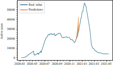
Figure 4 provides an example that will help the reader gain a greater understanding of the error distribution; in the case of a one-week prediction horizon, aggregated metrics can be provided using its absolute error to prevent sign compensation. Figure 5 illustrates the mean value of the absolute value of the relative error, along with the sample standard deviation of its distribution.
Figure 4. Relative error distribution in a one-week prediction
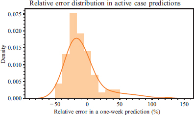
Figure 5. Mean of the absolute value of the relative error as a function of the prediction horizon
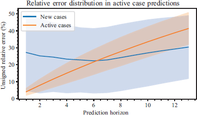
On average, the relative error in the number of new COVID cases is at 25 %. In the prediction of the number of active cases, the error is normally under 10 % for forecasts in the not distant future (under a week), when the limit is crossed, the growth is linear. Part of this uncertainty is caused by the variability of human reaction, which can be magnified by the geometric dynamics inherent to epidemiological processes.
4. Acknowledgments
The authors Lilia Muñoz and Vladimir Villarreal are members of the National Research System (SNI). This research was funded by Secretaria Nacional de Ciencia, Tecnología e Innovación (SENACYT Panamá) under Grant number 48-2020-COVID19-045.
5. Conclusions
Forecasting the transmission of the virus is highly complex because the scenario is dynamic; numerous factors intervene, such as the measures being implemented by the government at a particular point in time, the percentage of people that are vaccinated, the spread of new variations, etc.
The proposed system consists of an SIR model and a long short-term memory (LSTM) artificial recurrent neural network. It is capable of making forecasts 4–8 months ahead in order to enable the Panamanian government to manage the pandemic and curb the transmission rate. Thanks to the incorporation of the expert system, it is possible to introduce new variables into the model once they are known, e.g., new contingency measures. The combination of models in this proposal makes the system’s results interpretable. The system not only has the capacity to provide a clear picture of the current situation of the pandemic but is also able to forecast its evolution. The mean squared error in terms of the number of positive cases has been estimated to be around 18% and 22% for the active and new cases respectively in the 2-week predictions.
Future work will include the analysis of more complex compartmental models, as well as longer-term predictions.
References
Abadi, M., Agarwal, A., Barham, P., Brevdo, E., Chen, Z., Citro, C., Corrado, G. S., Davis, A., Dean, J., Devin, M., Ghemawat, S., Goodfellow, I., Harp, A., Irving, G., Isard, M., Jia, Y., Jozefowicz, R., Kaiser, L., Kudlur, M., Levenberg, J., Mané, D., Monga, R., Moore, S., Murray, D., Olah, C., Schuster, M., Shlens, J., Steiner,B., Sutskever, I., Talwar, K., Tucker, P., Vanhoucke, V., Vasudevan, V., Viégas, F., Vinyals, O. Warden, P., Wattenberg, M., Wicke, M., Yu, Y., and Zheng, X., 2015. TensorFlow: Large-Scale Machine Learning on Heterogeneous Systems. Software available from tensorflow.org.
Azouani, A., Olson, E., and Titi, E. S., 2014. Continuous data assimilation using general interpolant observables. Journal of Nonlinear Science, 24(2):277–304.
Bauch, C. T., 2005. Imitation dynamics predict vaccinating behaviour. Proceedings of the Royal Society B: Biological Sciences, 272(1573):1669–1675.
Bertozzi, A. L., Franco, E., Mohler, G., Short, M. B., and Sledge, D., 2020. The challenges of modeling and forecasting the spread of COVID-19. Proceedings of the National Academy of Sciences, 117(29):16732–16738.
Casas, E. and Mateos, M., 2017. Optimal control of partial differential equations. In Computational mathematics, numerical analysis and applications, pages 3–59. Springer.
Castillo Ossa, L. F., Chamoso, P., Arango-Lépez, J., Pinto-Santos, F., Isaza, G. A., Santa-Cruz-González, C., Ceballos-Marquez, A., Hernández, G., and Corchado, J. M., 2021. A Hybrid Model for COVID-19 Monitoring and Prediction. Electronics, 10(7):799.
Chimmula, V. K. R. and Zhang, L., 2020. Time series forecasting of COVID-19 transmission in Canada using LSTM networks. Chaos, Solitons & Fractals, page 109864.
Corchado, J. M., Chamoso, P., Hernández, G., Gutierrez, A. S. R., Camacho, A. R., González-Briones, A., Pinto-Santos, F., Goyenechea, E., Garcia-Retuerta, D., Alonso-Miguel, M. et al., 2021. Deepint. net: A Rapid Deployment Platform for Smart Territories. Sensors, 21(1):236.
Daza-Torres, M. L., Capistrán, M. A., Capella, A., and Christen, J. A., 2021. Bayesian sequential data assimilation for COVID-19 forecasting. arXiv preprint arXiv:2103.06152.
Engbert, R., Rabe, M. M., Kliegl, R., and Reich, S., 2021. Sequential data assimilation of the stochastic SEIR epidemic model for regional COVID-19 dynamics. Bulletin of mathematical biology, 83(1):1–16. Hethcote, H. W., 1976. Qualitative analyses of communicable disease models. Mathematical Biosciences, 28(3–4):335–356.
Hethcote, H. W., 1989. Three basic epidemiological models. In Applied mathematical ecology, pages 119–144. Springer.
Kabir, K. A. and Tanimoto, J., 2019. Dynamical behaviors for vaccination can suppress infectious disease-A game theoretical approach. Chaos, Solitons & Fractals, 123:229–239.
Kabir, K. A. and Tanimoto, J., 2020. Evolutionary game theory modelling to represent the behavioural dynamics of economic shutdowns and shield immunity in the COVID-19 pandemic. Royal Society open science, 7(9):201095.
Kermack, W. O. and McKendrick, A. G., 1927. A contribution to the mathematical theory of epidemics. Proceedings of the Royal Society of London. Series A, Containing papers of a mathematical and physical character, 115:700–721.
Kermack, W. O. and McKendrick, A. G., 1932. A contribution to the mathematical theory of epidemics, part. II. Proceedings of the Royal Society of London. Series A, Containing papers of a mathematical and physical character, 138:55–83.
Kermack, W. O. and McKendrick, A. G., 1933. A contribution to the mathematical theory of epidemics, part. III. Proceedings of the Royal Society of London. Series A, Containing papers of a mathematical and physical character, 141:94–112.
Kuperman, M. and Wio, H., 1999. Front propagation in epidemiological models with spatial dependence. Physica A: Statistical Mechanics and its Applications, 272(1–2):206–222.
Le Gruenwald, S. and Jain, S. G., 2021. Leveraging Artificial Intelligence in Global Epidemics. Elsevier.
Li, H., Peng, R., and Wang, Z. A., 2018. On a diffusive susceptible-infected-susceptible epidemic model with mass action mechanism and birth-death effect: Analysis, simulations, and comparison with other mechanisms. SIAM Journal on Applied Mathematics, 78(4), 2129–2153. https://doi.org/10.1137/18M1167863.
Markowich, P. A., Titi, E. S., and Trabelsi, S., 2016. Continuous data assimilation for the three-dimensional Brinkman-Forchheimer-extended Darcy model. Nonlinearity, 29(4):1292.
Mondaini, R. P., 2020. Trends in Biomathematics: Modeling Cells, Flows, Epidemics, and the Environment. Springer.
Ozturk, T., Talo, M., Yildirim, E. A., Baloglu, U. B., Yildirim, O., and Acharya, U. R., 2020. Automated detection of COVID-19 cases using deep neural networks with X-ray images. Computers in Biology and Medicine, page 103792.
Perc, M., Gorišek Miksić, N., Slavinec, M., and Stožer, A., 2020. Forecasting covid-19. Frontiers in Physics, 8:127.
Presentaciones Covid-19 - Ministerio de Salud, Gobierno de Panamá Ministerio de Salud, Gobierno de Panamá http://www.minsa.gob.pa/informacion-salud/presentaciones-covid-19-detalles. (Accessed on 05/20/2021).
Suo, J. and Li, B., 2020. Analysis on a diffusive SIS epidemic system with linear source and frequency-dependent incidence function in a heterogeneous environment. Math. Biosci. Eng., 17(1):418–441.
Tanimoto, J., 2021. Sociophysics Approach to Epidemics, volume 23. Springer Nature.
Tröltzsch, F., 2010. Optimal control of partial differential equations: theory, methods, and applications, volume 112. American Mathematical Soc.
Wang, S., Yang, X., Li, L., Nadler, P., Arcucci, R., Huang, Y., Teng, Z., and Guo, Y., 2020. A Bayesian Updating Scheme for Pandemics: Estimating the Infection Dynamics of COVID-19. IEEE Computational Intelligence Magazine, 15(4):23–33.
Yousaf, M., Zahir, S., Riaz, M., Hussain, S. M., and Shah, K., 2020. Statistical analysis of forecasting COVID-19 for upcoming month in Pakistan. Chaos, Solitons & Fractals, 138:109926.