
Regular Issue, Vol. 11 N. 1 (2022), 97-109
eISSN: 2255-2863
DOI: https://doi.org/10.14201/adcaij.27955
|
ADCAIJ: Advances in Distributed Computing and Artificial Intelligence Journal
Regular Issue, Vol. 11 N. 1 (2022), 97-109 eISSN: 2255-2863 DOI: https://doi.org/10.14201/adcaij.27955 |
A Study on the Impact of DE Population Size on the Performance Power System Stabilizers
Komla Agbenyo Folly, and Tshina Fa Mulumba
University of Cape Town, South Africa
ABSTRACT
The population size of DE plays a significant role in the way the algorithm performs as it influences whether good solutions can be found. Generally, the population size of DE algorithm is a user-defined input that remains fixed during the optimization process. Therefore, inadequate selection of DE population size may seriously hinder the performance of the algorithm. This paper investigates the impact of DE population size on (i) the performance of DE when applied to the optimal tuning of power system stabilizers (PSSs); and (ii) the ability of the tuned PSSs to perform efficiently to damp low-frequency oscillations. The effectiveness of these controllers is evaluated based on frequency domain analysis and validated using time-domain simulations. Simulation results show that a small population size may lead the algorithm to converge prematurely, and thus resulting in a poor controller performance. On the other hand, a large population size requires more computational effort, whilst no noticeable improvement in the performance of the controller is observed.
KEYWORDS
damping ratio; differential evolution; low-frequency oscillations; population size; power system stabilizer
1. Introduction
The basic function of a Power System Stabilizer (PSS) is to improve the damping of the system so that the transfer capability of the system could be extended. Generally, PSS is designed around the nominal operating condition using conventional methods such as root-locus, phase compensation, etc. (Kundur et al., 1989). However, PSSs designed using these approaches cannot guarantee the system’s stability due to the existence of nonlinearities in the system and the fact that the operating conditions are constantly varying. Over the past few years, optimal tuning of PSS parameters using artificial intelligence techniques such as genetic algorithms (GAs) and its variants, particle swarm optimization (PSO), population-based incremental learning (PBIL), differential evolution (DE), etc., has received increasing attention (Peng & Wang, 2018; Bibaya & Liu, 2016; Soeprijanto et al., 2016; Shafiullah et al., 2017; Abdel – Magid et al., 1999; Sheetekela & Folly, 2009a and 2009b; Folly, 2005; Shayeghi et al., 2010; Mitra et al., 2009; Mulumba & Folly, 2011). Among these algorithms, DE has proven to be a simple and yet powerful algorithm in solving real-valued optimization, and thus ranking among the best competing algorithms in numerous evolutionary computation (EC) algorithm tournaments (Price, 1997; Das & Suganthan, 2011). As a result, DE is used in this work to optimally tune PSS parameters. Like many other EC algorithms, the performance of DE is highly sensitive to the settings of its control parameters such as population size, mutation factor, and crossover probability. Inappropriate settings of these parameters could have a negative impact on the performance of the algorithm. (Storn & Price, 1997; Vesterstroem & Thomsen, 2004) have suggested some guidelines for selecting DE’s control parameters to achieve good performance of the algorithm. These guidelines were derived from some investigations conducted by the authors; however, when it comes to PSS tuning, these guidelines do not always yield expected outcomes because of the problem characteristics and the objective functions. Therefore, it is recommended that these settings be tuned on a specific problem and a trial-and-error basis (Mulumba, 2012; Eltaeib & Mahmood, 2018). Recent research focused on adaptively finding suitable settings for the crossover probability and the mutation factor which led to the so-called adaptive DE and self-adaptive DE algorithms (Brown et al., 2016; Mohamed, 2017; Brest et al., 2006; Brest et al., 20010; Lui & Lampinen, 2005; Suganthan & Qin, 2005; Duan et al., 2019; Georgioudakisa & Plevris, 2020). On the other hand, the effect of the DE’s population size on DE’s performance has not received much attention (Teo, 2006; Mallipeddi & Suganthan, 2008). Often, DE population size is specified by the user and is not given much attention and remains fixed during the run. However, the population size plays an important role in the performance of the algorithm. A small population size could lead to premature convergence with a higher probability of stagnation (i.e., an instance where the optimization process no longer progresses to allow the population to converge, instead it remains diverse) (Mallipeddi & Suganthan, 2008). To overcome this drawback, a large population size could be used. However, using a large population size will require significant computational effort and time without necessarily improving the algorithm’s performance (Montgomery, 2010; Mulumba & Folly, 2020; Mulumba, 2012). This paper investigates the impact of population size on the performance of DE when applied to the optimal tuning of PSSs and provides new insights into the relationship between the population size and the performance of DE-based controllers. Furthermore, we have also investigated whether the number of function evaluations affects the performance of the algorithm and hence the controller. It is shown that a large population size does not necessarily translate to a better damping ratio in terms of controller performance. Therefore, the relationship between damping ratio and population size is not linear. The simulation results also suggested that having more function evaluations will not necessarily lead to a better damping ratio if the size of the population is not appropriately chosen.
The paper is organized as follows: Section 2 presents the overview of DE; section 3 deals with the power system network used in the design; section 4 is concerned with the problem formulation and PSS design; section 5 discussed the simulation results and section 6 is concerned with the conclusions.
2. Overview of DE
Differential evolution (DE) is a population-based algorithm that has been applied to solve several optimization problems in engineering with great success. (Storn & Price, 1997) were the first to propose DE as an efficient, simple, and robust global optimization tool (Mulumba & Folly, 2011; Price, 1997; Das & Suganthan, 2011; Mitra et al., 2009; Storn & Price, 1997; Vesterstroem & Thomsen, 2004; Mulumba, 2012; Eltaeib & Mahmood, 2018). Some features of DE are (a) ease to use and efficiency in memory utilization and (b) flexibility in designing mutation distribution. Compared to many other evolutionary algorithms, DE is seen to perform better in terms of robustness, speed of convergence, etc. (Das & Suganthan, 2011; Mulumba, 2012).
2.1. Initialization
DE’s population is made of Np candidate solutions. Each candidate is a D dimensional real – valued vector where D is the number of variables to be optimized. The ith trial solution is denoted Xi,g = [xj,i,g] where j=1,2,…,D and «g» is the generation. The parameters of the vector are initialized within the specified upper and lower bounds xjU and xjL, respectively, such that xjL≤xj,i,g ≤ xjU.
The steps that DE follows at each generation g, are described below.
2.2. Mutation
Mutation in DE is used to assist with random perturbation on the population (Mulumba, 2012). In this process, a mutant vector is generated for each population member as given below:
where F is the mutation factor that controls the amplification of second term in Eq. (1) and F [ 0 2]. Indices r0, r1 and r2 are randomly chosen integers in the range [1, Np] (Storn & Price, 1997; Mulumba, 2012).
Note that Eq. (1) above is the basic mutation strategy. Several other mutation strategies could be used. Interested reader could read (Das & Suganthan, 2011; Mulumba, 2012; Eltaeib & Mahmood, 2018; Mallipeddi & Suganthan, 2008).
2.3. Crossover
Using a binomial crossover, the target vector is combined with the mutant vector to yield a D-dimensional trial vector as given in Eq. (2).
where CR [0, 1] is the crossover rate and randj is a random number between [0, 1]. jrand is the random mutant parameter that ensures that the trial vector receives at least one element from the mutant vector; otherwise, no new parent vector is generated and the population will remain the same.
2.4. Selection
In DE, the greedy selection strategy is generally adopted according to Eq. (3). According to this equation, if the fitness function of Ui,g is bigger than or equal to the fitness function of Xi,g (for maximization problem), then Ui,g is set to Xi,g+1. Otherwise, Xi,g is retained
2.5. Population Size
The population size plays an important role in the performance of the algorithm. A small population size could lead to premature convergence with a higher probability of stagnation. Previously, DE population size was largely treated as problem independent. Recent research has shown that the population size should be treated as problem dependent (Teo, 2006; Mallipeddi & Suganthan, 2008). For small population size, DE could converge too early. To overcome this problem, a larger population size could be used. Nonetheless, using a large population will necessitate large computational effort and time without necessarily improving the algorithm’s performance. For efficient performance, it was suggested in (Storn & Price, 1997) that a population size between 7.D and 10.D should be used. In our opinion, the issue of population size has not received the attention it deserves as most research so far has been primarily concerned with adaptive DE or self-adaptive DE (Brown et al., 2016; Mohamed, 2017; Brest et al., 2006; Brest et al., 20010; Lui & Lampinen, 2005; Suganthan & Qin, 2005; Duan et al., 2019; Georgioudakisa & Plevris, 2020). In this study, the parameters of the PSSs are optimally tuned when DE’s population is varying.
3. Power System Model
The two-area, 4- machine benchmark power system model is used in this study. The system consists of four identical machines (see Figure 1). The machines are modeled using detailed differential equations (6th order). Simple exciter systems are installed on the generators. The dynamics of the system are modeled by nonlinear differential equations. These equations are then linearized around the nominal operating condition. The state-space equations may be found in (Sheetekela & Folly, 2009a; Sheetekela & Folly, 2009b; Mulumba, 2012).
Figure 1. Power system model
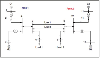
The system contains two local modes and one inter-area mode. In this paper, only the inter-area modes will be discussed since they are the most critical modes.
4. PSS Parameter Tuning
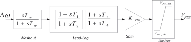
We are primarily concerned with the optimization of PSS’s parameters such that the controllers can adequately provide the necessary damping to the oscillation modes over the ranges of operating conditions considered. Note that the frequencies of oscillations considered are between 0.2 to 3 Hz. Several input signals such as speed deviation, electrical output, could be used as PSS input. However, for simplicity, we assumed speed deviation as input. The PSS is made of a gain Kp, lead-lag time constants, and a reset or washout block as shown in Figure 2. From a design perspective, the washout is needed to prevent the PSS from operating under steady steady-state conditions. The value of Tw is not critical and is selected in this study to be 10 sec (Kundur et al., 1989; Mitra et al., 2009; Mulumba & Folly, 2011; Mulumba, 2012). A limiter is provided to limit the PSS output to specified values. The limiter will be useful only under large disturbances, where the output of the PSS could be large.
Figure 2. Block diagram of a typical PSS
In total there are 10 variables to optimize, i.e., five variables for each area of Figure 1. This means the problem dimension is 10. Since generator G1 is identical to G2, the PSS parameters for these two generators were set to have the same values. The same applies to G3 and G4.
The following are the constraints that have been applied to these variables:
The objective function is given in Eq. (6), where the minimum damping ratio is maximized over selected operating conditions
where i = 1,2, …., n eigenvalues and j = 1,2,…, m operating conditions
In this work, we consider a range of populations varying from 10 (D) to 200 (20.D). As for the iterations/generations, DE was run for a total of 200 generations.
The parameters of DE are given below:
Population size: 10 - 200
Generation: 200
Mutation factor F: 0.90
Crossover probability CR: 0.95
CR and F values have been selected after some careful investigations as discussed in (Mulumba, 2012; Mulumba & Folly, 2020) and the above values were found to be the most suitable.
We have considered several operating conditions during the design of the PSSs, however, for the time domain simulations, only three cases are discussed in this paper where the tie-line number between the two areas was maintained at 2. Table 1 lists the three case studies considered in this paper. In case 1, real power of 1.0 pu is transferred from area 1 to area 2 whereas in case 2, this power was increased to 2.0 p.u. In case 3, the active power transferred from area 1 to area 2 was further increased to 3.0. p.u. For case 1, the inter-area modes oscillate at a frequency of 0.78 Hz with a damping ratio of 0.1%. Hence, these oscillations are sustained for a long period. For case 2, the inter-area modes were found to be unstable which is characterized by a negative damping ratio of -0.9% hence growing oscillations of frequency of 0.77 Hz are observed in the system. For case 3, the inter-area modes were further destabilized as the corresponding poles moved further into the right-hand side of the s-plane.
Table 1. Operating conditions considered
Case |
Real power (p.u) |
Tie-line no. |
1 |
1.0 |
2 |
2 |
2.0 |
2 |
3 |
3.0 |
2 |
5. Simulation Results
5.1. Modal Analysis
Since inter-area modes are more critical than local modes, in our discussion, we will only concentrate on the inter-area modes and ignore the local modes. Table 2 shows the results for 10 independent runs. The ‘best damping’ referred to the maximum damping obtained from 10 independent runs. ‘Mean’ represents the average of the best damping ratios over the 10 independent runs. Table 2 shows that as the population increased, the damping ratio also increased up to a certain population size (i.e., 150 which is 15.D). A further increase in the population size to 200 (20.D) does not yield any improved results. When the population is set to 10 (D), the lowest damping ratio was recorded which translates to the worst performance of the DE algorithm and hence the controller. This is expected since when population size is low, the diversity in the population is reduced and this leads to the algorithm converging prematurely. When DE population size is 30 (3.D), the best damping ratio increased by 40.87% compared to when the population size was D. When the population size increased to 50 (5.D), the best damping has further improved by about 10.46 % compared to the 3.D case. Therefore, the total improvement in damping is about 51.33% higher when compared to the case when the population size was set to D. From Table 2 one can see that for the population size of 50 (5.D), the algorithm converged to a damping ratio of 26.94 % and has a mean damping ratio of 23.01%. For 7.D, the best damping ratio was reduced slightly by about 3.53% compared to the 5.D case. For a population size of 100 (10.D), the best damping ratio has increased slightly by about 2.77% compared to 7.D. However, compared to 5.D, it can be seen that the damping ratio of 10.D has slightly reduced by about 0.85%. This means that when the population size is 5.D, the algorithm seems to perform slightly better in terms of damping ratio than when the population is 10.D. In other words, a population of 5.D is similar or slightly better than a population of 10.D in terms of damping ratio. Therefore, if one were to design the controller, it will make sense to use the smaller population size of 5.D than 10.D as it will save computational effort and time. For a population of 150 (15.D), the algorithm converges to the best damping ratio of 27.4% which is the highest overall and has a mean value of 24.58%. When the population is increased from 15.D to 20.D, the best damping ratio reduces by 5%. The results suggest that a large population size may not necessarily translate to a better performance of the controller.
Table 2. Best and Mean damping ratio and Std Dev.
Population size |
Best |
Mean |
Std. Dev. |
10 (D) |
0.1780 |
0.1610 |
0.0163 |
30 (3D) |
0.2439 |
0.2268 |
0.0224 |
50 (5D) |
0.2694 |
0.2301 |
0.0110 |
70 (7D) |
0.2599 |
0.2214 |
0.0235 |
100 (10D) |
0.2671 |
0.2254 |
0.0322 |
150 (15D) |
0.2740 |
0.2458 |
0.0282 |
200 (20D) |
0.2603 |
0.2231 |
0.0267 |
When we look at the standard deviation, one can see that the standard deviation of 10.D is the highest. This means that the data points for this population size are spread out over a wide range of values. The smallest standard deviation is obtained when the population size is 5.D which means the data points are concentrated around the mean.
Figure 3 shows the fitness values (damping ratio) of all populations that were investigated. For a small population size (10), the algorithm lost its diversity early in the run and converged too early to a sub-optimal solution (i.e., damping ratio less than 0.2). This means that the controller will perform poorly. Although the population size of 30 performed slightly better than that of 10, it also converged to a sub-optimal solution after about 80 generations. This means that for these two population sizes (10 & 30), DE experiences a premature convergence. As the population is increased to 50, 70, and 150, the algorithm was able to explore the search space further and thus the controller was able to provide better or similar damping ratios. However, when the population size is increased to 200, this did not yield any further improvement in the damping ratio after 200 generations (see Figure 4). This suggests that if the population size is too large, it is not necessarily beneficial to the algorithm as the performance of the controller is not necessarily improved.
Figure 3. Damping ratio vs generation
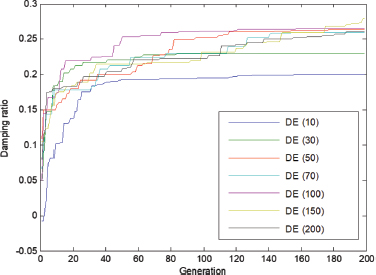
Figure 4. Damping ratio vs population size

We have also investigated whether the number of function evaluations affects the performance of the algorithm and hence the controller. It should be mentioned that the maximum number of function evaluations (FEs) in this study is 40000 and the lowest FEs is set to 2000 which corresponds to the smallest population size of 10 (D). Let assume that we set the function evaluations to be 2000. Then the different population sizes will be allocated to different generations to reach this target. For example, the population sizes of 10, 30, 50, 70, 100, 150, and 200 will reach this FEs after about 200, 67, 40, 29, 20, 13, and 10 generations, respectively. It is clear from Figure 3 that for the same function evaluations, all the population sizes that are bigger than 10, provide a better damping ratio than the population size of 10. It is observed from this Figure that, even if the number of FEs was to be increased for the population size of 10, one could not increase the damping ratio due to the fact the population size was too small. However, for other population sizes, the damping ratio increase as the number of function evaluations increased. Note, however, that for the population size of 30, the damping ratio improves only up to about 80 generations (2400 function evaluations). After that, no improvement could be observed. This suggests that having more function evaluations will not necessarily lead to better results if the size of the population is not appropriately chosen. It is observed that the population size of 100 provides the best overall damping than the rest until about the 180th generation when it was overtaken by the population size of 150. It took the latter relatively long time before it could provide the best overall damping after about 27000 FEs.
The population size of 200 was not able to provide better damping than the population sizes of 50 (10000 function evaluations), 100 (20000 function evaluations,) and 150 (30000 function evaluations), respectively even after 200 generations (40000 function evaluations). This suggests that a large population size with more function evaluations does not necessarily translate to a better damping ratio in terms of controller performance. Therefore, the relationship between damping ratio and population size is complex and nonlinear. It is therefore important to carefully select the appropriate population for a given problem.
5.2. Time Domain Simulation under Small Disturbance
The results of the modal analysis are validated by performing time-domain simulations. In all the simulations, a 10% step change in the voltage reference of the generator G2 was considered. Because the responses of all the population sizes cannot be put together, they have been split into two Figures for each case (i.e., Figs 5-6 and Figs 7-8).
Figure 5 (population sizes 10-70) and Figure 6 (population sizes 100-200) show the rotor speed deviation responses for case 1. For Figure5, the population size of 50 seems to settle quicker than the rest of the populations. The population size of 30 has the smallest undershoot but has some offset (i.e., did not settle to zero). The responses in Figure 6 seem to have overall smaller overshoots and undershoots than the ones in Figure 5. This suggests that the responses in Figure 6 have on average better damping. Overall, the population size of 200 has the fastest settling time.
Figure 5. Rotor speed deviation for case 1 (population sizes 10, 30 50 & 70)
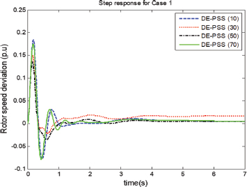
Figure 6. Rotor speed deviation for case 1 (population sizes 100, 150 & 200)
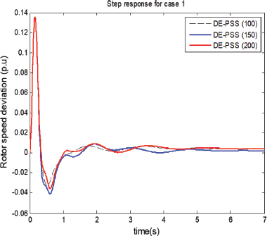
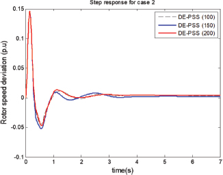
Figure 7 (population sizes 10-70) and Figure 8 (population sizes 100-200) show the rotor speed deviation response for case 2. Figure7 is similar to Figure 5, except that the open-loop damping of Figure 7 has deteriorated because of the increase in real power transfer which has destabilized the system. This is the reason why the responses in Figure 7 have higher overshoots and undershoots when compared to Figure5. Again, for this case, the population size of 50 seems to settle quicker than the rest of the populations and the population size of 30 has the smallest undershoot, but has some offset (i.e., did not settle to zero). For Figure 8, the population sizes of 100, 150, 200 which provide more damping to the system have overall smaller overshoots and undershoot than those in Figure 7. Overall, the population of 200 has the fastest settling time, followed by the population size of 100. We note that the population size of 150 which shows good performance in terms of modal analysis did not perform extraordinarily as one would have expected when it comes to time-domain simulations.
Figure 7. Rotor speed deviation for case 2 (population sizes 10, 30 50 & 70)
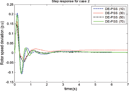
Figure 8. Rotor speed deviation for case 2 (population sizes 100, 150 & 200)
6. Conclusions
This paper investigates the effect of population size on DE’s performance when applied to the optimal tuning of PSS’s parameters. It is observed that the selection of appropriate population size can have a positive impact on the DE algorithm, and, and hence the performances of the PSSs. It was shown that if the population size is too small this could lead the algorithm to converge prematurely and thus resulting in poor controller performance. Notwithstanding, if the population size is too large, more computational effort and time are required, but no noticeable improvement in the performance of the algorithm or the controller is observed. Therefore, there is a need for a trade-off between computational effort and performance. Frequency and time-domain simulations have been presented to show the impact that the population size has on the performance of DE. It was found that for a good performance of the algorithm and the controllers, the appropriate population size should be between 5D (50) and 15D (150). A higher populations size of 20D (200) did not seem to give an extra edge in improving the controller’s performance in terms of damping ratio. Time-domain simulations show that some of the population sizes that did not perform well under modal analysis did relatively well under time-domain analysis. More investigations are needed in the future to get a better understanding of this phenomenon.
7. Acknowledgements
This work was based on the research supported in part by the National Research Foundation of South Africa under Grants UID 118550.
References
Abdel – Magid, Y. L., Abido, A., and Mantaurym, H., 1999. Simultaneous stabilization of Multimachine Power System via genetic algorithm. In IEEE Trans. Power Sys., pages 1428–1438.
Bibaya, L., and Liu, C., 2016. Optimal tuning and placement of power system stabilizers based eigenvalues. In Indonesia Journal of Elec. Eng. And Comput. Sciences, pages 273–281.
Brest, J., Greiner, S., Boskovic, B., Mernik, M., and Zumer, V., 2006. Self-adapting control parameters in differential evolution: a comparative study on numerical benchmark problems. In IEEE Trans. on Evolutionary Computation, pages 646–657.
Brest, J., Boškovič, B., and Žumer, V., 2010. An improved self-adaptive differential evolution algorithm in single-objective constrained real-parameter optimization. In Proc. of the IEEE Congress on evolutionary computation.
Brown, C., Jin, Y., Leach, M., and Hodgson, M., 2016. µJADE: Adaptive Differential Evolution with a Small Population. In Soft Computing, pages 4111–4120.
Das, S., and Suganthan, P. N, 2011. Differential evolution: a survey of the state-of-the-art. in IEEE Trans. On Evol. Comput., pages 4–31.
Duan, M., Yang, H., Wang, S., and Liu, Y., 2019. Self-adaptive Dual-strategy Differential Evolution Algorithm. In Plos One 14(10). https://doi.org/10.1371/Journal.pone.0222706.
Eltaeib, T., and Mahmood, A., 2018. Differential evolution: a survey and analysis. Applied Sciences, MDPI. 7, 1945. https://doi.org/10.3390/app8101945.
Folly, K. A., 2005. Multimachine power system stabilizer design based on a simplified version of genetic algorithm combined with learning. In Proc. of International Conference on Intelligent Systems Application to Power Systems (ISAP).
Folly, K. A., and Mulumba, T., 2020. Impact of population size on the performance of DE-based Power System Stabilizers. In proc. of 24th European conference in Artificial Intelligence (ECAI), workshop on artificial- intelligence-in-power-and-energy-systems-(AIPES), paper ID No.8, 2020.
Georgioudakisa M., and Plevris, V., 2020. On the Performance of Differential Evolution Variants in Constrained Structural Optimization. In Procedia Manufacturing, pages 371–378.
Kundur, P., Klein, M., Rogers G., and Zywno, M., 1989. Application of power system stabilizers for enhancement of overall system stability. In IEEE Trans. Power Syst., pages 614–626.
Lui J., and Lampinen, J., 2005. A Fuzzy adaptive differential evolution algorithm. In Soft Computation: Fusion Found Method Appl., pages 448–462.
Mallipeddi R., and Suganthan, P. N., 2008. Empirical Study on the Effect of Population Size on Differential. In Proc. of IEEE Congress on Evolutionary Computation.
Mitra, P., Yan, C., Grant, L., Venayagamoorthy, G. K., and Folly, K., 2009. Comparison study of population-based techniques for power system stabilizer design. In Proc. of the 15 th Int. conf. on Intelligent, Curitiba, Brazil.
Mohamed, A. W., 2017. Solving large-scale global optimization problems using enhanced adaptive differential evolution algorithm’, In Complex Intell. Syst., pages 205–231.
Montgomery, J., 2010. Crossover and the different faces of differential evolution searches. In Proc. of IEEE Congress on Evolutionary Computation.
Mulumba, T., and Folly. K. A., 2011. Design and comparison of Multi-machine Power System Stabilizer based on Evolution Algorithms. In Proc. of. Universities’ Power Engineering Conference (UPEC).
Mulumba, F., 2012. Application of Differential Evolution to Power System Stabilizer Design. MSc Dissertation, University of Cape Town, Cape Town.
Mulumba, T. F., and Folly, K. A., 2020. Application of Evolutionary Algorithms to Power System Stabilizer Design. In Implementations and Applications of Machine Learning, Studies in Computational Intelligence 782, Subair S, Thron, C, Eds., pages 29–62. Springer.
Peng, S., and Wang, Q., 2018. Power system stabilizer parameters optimization using immune genetic algorithm. In IOP Conf. Series: Materials Sci. and Eng., 394. https://www.doi.org/10.1088/1757-899X/394/4/042091.
Price, K. V., 1997. Differential evolution vs. the functions of the 2nd ICEO. In Proc. IEEE Int. Conf. Evol. Comput. pages 153–157.
Shafiullah, Md., Juel Rana, Md., and Abido, M. A., 2017. Power system stability enhancement through optimal design of PSS employing PSO. Fourth Int. Conf. on Adv. In Elec. Eng. (ICAEE).
Shayeghi, H., Shayanfar, H. A., Safari, A., and Aghmasheh, R., 2010. A robust PSSs design using PSO in a multi-machine environment. Energy Convers. and Manag. pages 696–702.
Sheetekela, S., and Folly, K., 2009a. Multimachine power system stabilizer design based on evolutionary algorithms, The 44th international Universities. Power Engineering Conference (UPEC).
Sheetekela, S. P. N., and Folly, K. A., 2009b. Optimization of Power System Stabilizers using Genetic Algorithm Techniques based on Eigenvalue analysis. 18th Southern African Universities’ Power Engineering Conference (SAUPEC).
Soeprijanto, A., Putra, D. F. U., Fenno, O., Suyanto, Ashari, H. S. D., and Rusilawati., 2016. Optimal tuning of PSS parameters for damping improvement in SMIB model using random drift PSO and network reduction with losses concept. In Int. Seminar of Intelligent Technology and Appl. (ISITIA) 2016.
Storn, R., and Price, K., 1997. Differential Evolution: a simple and effective heuristic for global optimization over continuous spaces. Journal of global optimization, pages 341–359.
Suganthan, P. N., and Quin, A. K., 2005. Self-Adaptive Differential Evolution Algorithm for numerical optimization. In Proc. of the IEEE Congres on Evolutionary Computation.
Teo, J., 2006. Exploring dynamic self-adaptive populations in differential evolution. In Soft. Comput. pages 673–686.
Vesterstroem J., and Thomsen, R., 2004. A comparative study of differential evolution, particle swarm optimization, and evolutionary algorithms on numerical benchmark problems. In Proc. of the IEEE Congress on Evolutionary Computation.
Author’s Biography

Komla Agbenyo Folly received the B.Sc. and M.Sc. degrees in electri-cal engineering from Tsinghua University, Bei jing, China, in 1989 and 1993, respectively, and the Ph.D. degree in electrical engineering from Hiroshima University, Japan, in 1997. From 1997 to 2000, he worked with the Central Research Institute of Electric Power Industry (CRIEPI), Tokyo, Japan. He is currently a Professor with the Department of Electrical Engineering, University of Cape Town, Cape Town, South Africa. In 2009, he received a Fulbright Scholarship and was Fulbright Scholar with the Missouri University of Science and Technology, Rolla, MO, USA. His research interests include power system stability, control and optimization, HVDC modeling, grid integration of renewable energy, application of computational intelligence to power systems, smart grids, and power system resilience. He is a member of the Institute of Electrical Engineers of Japan (IEEJ), Senior Member of the IEEE a and a Fellow of the South African Institute of Electrical Engineers (SAIEE).

Tshina Fa Mulumba received his BSc and MSc degrees in Electrical Engineering from the University of Cape Town, South Africa, in 2009 and 2013, respectively. From 2013 to 2019 he was with ESP consulting group where he was employed as a Senior Engineer. In 2019, he joined the Development Bank of Southern Africa as a Principal Investment Officer. His research interests include operation, control and optimization, machine learning, and application of Evolutionary algorithms to power systems, sustainable investments in the energy sector across sub-Saharan Africa.