Figure 1. Convex Function of Gradient Descent. (Retrieved February 4, 2022, from https://blog.paperspace.com/intro-to-optimization-in-deep-learning-gradient-descent/)
ADCAIJ: Advances in Distributed Computing and Artificial Intelligence Journal
Regular Issue, Vol. 11 N. 3 (2022), 263-283
eISSN: 2255-2863
DOI: https://doi.org/10.14201/adcaij.27822
Learning Curve Analysis on Adam, Sgd, and Adagrad Optimizers on a Convolutional Neural Network Model for Cancer Cells Recognition
José David Zambrano Jaraa and Sun Bowenb
a,b School of Computer Science and Technology, Harbin University of Science and Technology, Harbin, China
✉ macwolfz@gmail.com, 1456174486@qq.com
ABSTRACT
Is early cancer detection using deep learning models reliable? The creation of expert systems based on Deep Learning can become an asset for the achievement of an early detection, offering a preliminary diagnosis or a second opinion, as if it were a second specialist, thus helping to reduce the mortality rate of cancer patients. In this work, we study the differences and impact of various optimizers and hyperparameters in a Convolutional Neural Network model, to then be tested on different datasets. The results of the tests are analyzed and an implementation of a cancer classification model is proposed focusing on the different approaches of the selected Optimizers as the best method for the achievement of optimal results in accurately improving the detection of cancerous cells. Cancer, despite being considered one of the biggest health problems worldwide, continues to be a major problem because its cause remains unknown. Regular medical check-ups are not frequent in countries where access to specialized health services is not affordable or easily accessible, leading to detection in more advanced stages when the symptoms are quite visible. To reduce cases and mortality rates ensuring early detection is paramount.
KEYWORDS
health; medicine; cancer; detection; deep learning; technology; artificial intelligence; machine learning; image classification
1. Introduction
Convolutional Neural Networks (CNNs) have proven useful and have shown highly promising results in Computer-Aided Detection (CADe). The use of Deep Neural Networks minimizes the need for invasive procedures or testing, as well as prevent errors from missed diagnoses where a trained model acts as a second specialist observer, double-checking the results with the benefit that it can bear massive loads of cases in a matter of seconds.
With each advancement in technology, new methods arise, and old methods are refined, an example being CADe methods (Chan et al., 2020). Old methods are being more fine-tuned reaching new levels of precision and accuracy with the help of Deep Learning (Alzubaidi et al., 2021), while new methods are being developed by people around the world which helps in the development of new algorithms (Ozawa et al., 2020) for different models and architectures.
In recent years, new problems have emerged and new techniques have been developed to counteract (Johnson et al., 2021) said problems. Some problems are often associated with using datasets, such as having corrupted data, and or insufficient files. One way to solve this type of problem is by using Data Augmentation which has been proven to work (Shorten and Khoshgoftaar, 2019) by expanding datasets.
Data Augmentation is only able to help improve the dataset to an extent (Hussain et al., 2017), after that it might require different techniques for it to work (Camdemir et al., 2021) and interpret an unrepresentative dataset (More A., 2016) in case one exists.
In this study, the effects and interactions of parameters and tuning are presented, one of these parameters is the ‘Optimizer’, which updates the weight (Cheng et al., 2021) during Backpropagation.
The Optimizers chosen for this study were ADAM, ADAGRAD, SGD with momentum, and SGD+ Nesterov. The best result from these four optimizers has been tested further on, tuning its parameters for optimal results, allowing the creation of a more robust Lung Cancer Recognition Model.
1.1. Datasets
The main Dataset that was used in this research was ‘Mastorides SM. Lung and Colon Cancer Histopathological Image Dataset’, which is a collection of benign and cancerous tissue slides (Borkowski et al., 2019) divided on 5 classes for Lung and Colon cells.
In addition, the collections from two datasets, related to cancerous cells, were tested during this study, namely, the Collection of Textures in Colorectal Cancer Histology ‘Kather_texture_2016_image_tiles_5000’ (Kather et al., 2016), and Histological Images of Human Colorectal Cancer and Healthy Tissue (Kather et al., 2018) ‘NCT-CRC-HE-100K’.
1.2. Problem Approach
To take this approach, the first step was to research about different optimizers as background study, and to select the best options that would be used during this paper, that is, those which are the most suitable, in accordance with the selected database.
After selecting the optimizers, the next step was to prepare the information on a structure valid for the model to use. Initially, the slides from each class were separated into a new subset of Training, Validation, and Test, and the images were pre-processed for their further use to train and feed our model. Then, while defining the structure of the model, a set of hyperparameters have been tuned to seek the most effective values.
During the research, a set of different optimizers were used as well as various sets of hyperparameters values on the previously mentioned Datasets until optimal results were achieved. Once the model reaches a desirable amount of accuracy and loss, it is able to classify the different types of cells of the dataset, separating them into different folders according to his prediction.
Finally, a confusion matrix was created to display the results of the final model classifying performance after the test, showing a chart according the right predictions and errors on our Dataset.
2. Literature Review
2.1. Connection between Deep Learning and Predictive Medicine
The concept of Deep Learning stands for a new learning paradigm in Machine Learning, where a deep architecture model is created through a set of various consecutive layers, and each layer is specialized on extracting multiple features by applying a series of transformations. The goal of such models is to learn complicated and abstract representations of data such as pixels in an image which enter as an input into the first layer, to consequently send the processed output data as an input (Najafabadi et al., 2015) into its next layer.
In this study we use Convolutional Neural Networks (CNN), a class of artificial neural network, which is known for its high accuracy on Image Classification tasks, and it is proven to be very effective in the field of Preventing Medicine where an early detection of a disease is required for timely treatment, especially for patients diagnosed with cancer.
In some countries where a regular check-up is not necessarily frequent due to its cost, lack of specialized means such as equipment or personnel, they usually fail to detect signs and symptoms of cancer at its early stages. Machine Learning proposes diverse methods for approaching these challenges previously mentioned, revolutionizing Health Care field with the presence of artificial intelligence (AI) and precision medicine.
Patients with rare or unique responses to treatment can be identified easier by mixing high precision methods with the new Artificial Intelligence technologies. AI augments human intelligence by using advanced computation and inference to generate insights, support the system 's reasoning and learning capabilities, and facilitate decision-making process for medical personnel. According to recent literature, translating this convergence into clinical research helps address some of the most difficult challenges facing precision medicine, especially for those in which clinical information from patient symptoms (Johnson et al., 2021), clinical history, and lifestyles facilitate personalized diagnosis and prognosis.
The application of new Machine Learning methods and technologies in the field of medicine allows us to provide and adapt early preventive diagnostics and therapeutic strategies to each patient in an optimal and personalized manner. When implemented in health systems, machine learning algorithms can use these datasets to develop recognition or detection models, which, when implemented in healthcare systems, can aid in improving patient care, reducing diagnostic errors, supporting decision-making, and helping clinicians with Electronic Health Record (EHR) data extraction (Scholte et al., 2016) and documentation.
2.2. Deep Learning for illness Classification, Detection and Segmentation
With the advance of technologies, arise new and more complex algorithms for Classification, Detection and Segmentation methods based on Deep Learning, offering innovative approaches and tools for medicine specialists to assist in detecting cancerous cells, lesions and tumors in patients, allowing for a better diagnosis and treatment.
The effectiveness displayed by Neural Networks for task-specific sophisticated feature learning (Bengio, 2014) has helped to achieve high precision detection of illnesses such as tumor progression, where the affected area can be detected and circled inside a box (detection), or highlighted the contours (Segmentation), and separated according to which type of a disease it belongs to (classification).
In other words, the efficacy of molecular imaging diagnostics for the early diagnosis of cancer can be enhanced and the heavy workload of radiologists and physicians can be reduced, especially when there are subtle pathological changes that cannot be seen visually (Yong Xue et al., 2017).
Other studies have suggested the effectiveness of using Computer-Assisted Diagnostic Systems while undertaking tasks such as Colorectal cancer (CRC) screening (Taghiakbari et al., 2021) and prevention examinations.
During these examinations deep learning algorithms automatically extract diminutive (lesser than 5 mm) and small (lesser than 10 mm) polyp features (Tom et al., 2020). Besides, by implementing visualization Enhance methods such as blue-light imaging, narrow-band imaging (NBI), and i-Scan, it is possible to attain improved and reliable pathology predictions (Taghiakbari et al., 2021) during this process.
The massive advantages that Deep Learning has to offer to the medical field are quite evident, evolving to cover the 3 most important applications for image analysis in the medical field, such as target detection, segmentation, and classification, however, new opportunities also brought along with certain challenges. For example, the use of different Datasets on which deep learning models profoundly rely on, are limited and rather scarce, since the process for training these models require a massive load of data, or even by having large amounts of data, these datasets are still not fit enough for creating optimal and highly accurate models, so different strategies must be applied to improve the Accuracy and Loss of these models, and their inherent tools such as optimizers, which are studied in this research.
3. Optimizers
3.1. Stochastic Gradient Descent (SGD)
The main feature of the optimizer is that unlike the original algorithm, which was based on (Gradient Descent), where a series of calculations are made on the entire dataset, it takes into consideration a small subset of randomly chosen datasets.
As a result, the computing speed increases (Tom et al., 2020) while the storage requirements decrease. SGD updates the weights after seeing each data point instead of the entire dataset, however, it makes rather noisy jumps away from the optimal values since it is influenced by every individual input. The formula for every epoch and every sample on this algorithm is:
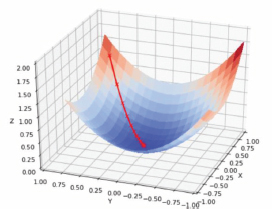
Where θ1), as an element of the domain of Real numbers represents the next position of the parameter of the objective function J(θ), which keeps updating through each training example to the opposite direction of the gradient of the objective function . Being this objective Function the gradient of J(θ) respect to θ, and α the learning rate, which reverse the direction of this gradient obtaining the direction of maximum descent (Elashmawi, 2019). In other words, As the position of the cost function gets smaller and smaller, the formula recounts the next position towards the steepest descent. (Figure 1)
Figure 1. Convex Function of Gradient Descent. (Retrieved February 4, 2022, from https://blog.paperspace.com/intro-to-optimization-in-deep-learning-gradient-descent/)
The training environments of high complexity in which Gradient Descent methods fail to work properly has led to the development of several new algorithms that complement technological advances (Zhou et al., 2020). One disadvantage of SGD is how it evenly scales the gradient in every direction (Keskar and Socher, 2017), turning the process of tuning the learning rates α fairly arduous. Besides, SGD Algorithm convergence rate is rather slow, due to the inherent propagate process that goes backward and forward for every record (Ruder, 2016). Another way of decrease the noise of SGD is to add the concept of Momentum (Bengio, 2012) to the model. The hyperparameters of the model may have the tendency of changing in one direction; with Momentum, the model can learn faster by minimizing the attention paid to details on the few examples that are being shown to it.
Where a fraction ‘γ’ (also called ‘momentum’, generally set to a value around 0.9) of the update vector is added to the current update velocity vector represented by ϑ, in order to attain a faster convergence and reduced oscillation. Calculating θ=θ-αϑ helps to find the most suitable value by iteratively obtaining the eigenvalues, where α is the drop coefficient, that is, the step size and the learning rate.
In other words, finding the magnitude of each drop. A larger coefficient leads to a greater difference in each calculation, while a smaller coefficient, causes a smaller difference, however, the iterative calculation time is relatively longer. The initial value of θ can be assigned randomly, as for example, the initial value can be set to 0. However, choosing to blindly ignore samples because they do not have typical features is reflected in a higher loss; to this end, an acceleration term is added.
Being ϑt) the velocity of time t and ϑt-1) the velocity of the previous time step, and representing gradient at the particular time ‘t’, and momentum γ is set a value of around 0.9 as well. This new Gradient has the particularity that when is close to the optimal value, or is near to the minimum value of the slope, the result of the gradient becomes negative, directing the gradient update back towards θt (Gylberth, 2018), allowing it to avoid oscillations. Nesterov acceleration presents some advantages over normal SGD with Momentum, where the gradient of future position is taken (Schmidt et al., 2018) instead of current position. In other words, the model gains momentum during training, so when it finds an odd example, because of the added momentum it does not pay too much attention to it.
Discarding it leads to a loss decrease that is not too abrupt as it is with normal SGD + Momentum (Ruder, 2016), this is where the weight updates are decelerated, so they become small again, allowing future examples to fine-tune the current model (Sutskever et al., 2013), updating the weights and bias rather dynamically (Figure 2).
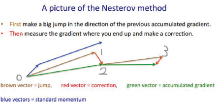
Figure 2. Nesterov method process (Retrieved on February 4, 2022 from https://towardsdatascience.com/gradient-descent-explained-9b953fc0d2c)
3.2. Adagrad
Adagrad adjusts the learning rate to the parameters, carrying out a set of small updates for recurrently features, and a bigger learning rate for uncommon features. The main idea of this algorithm is to keep in memory the sum of squares of the gradients with respective θi parameter up to a certain point.
Where θt,i is the current parameter value on i during every time step t, while θt+1,i is the updated parameter after one time step. η (ETA) value is usually set to 0.01, and ϵ representing a relatively small number used to ensure that the denominator is not 0 (usually on the order of 1e-8), Gt contains the gradient estimate at time step ‘t’ with relation to the parameters θi (Ruder, 2016), obtained as the partial derivative of the objective function respect to the parameter θi, and Gt,ii as a diagonal matrix where each diagonal element i,i is the sum of the squares of the gradients respect to θi up to time step t.
In other words, the learning rate is divided by the square root of all previously obtained gradients, the momentum concept is removed, while the learning rates are adjusted according to the parameters. This is unlike the other optimizers, where an update is performed for all parameters θ, instead of using a different learning rate for every parameter on each Epoch.
3.3. Adam
This method incorporates the momentum concept from «SGD with momentum» and adaptive learning rate from «Ada delta», as well as the best features of AdaGrad and RMSProp practices, making Adam suitable to handle sparse gradient gradients (Kingma and Ba, 2015) easily on noisy problems. Sparse gradients are, in essence, a way to shift the approach of the Original Past Gradient (OPG) from calculating gradient vectors only at observed points to computing gradients over the entire domain (Ye and Xie, 2012). This algorithm can obtain better results than many other optimizers in the field of deep learning. This was demonstrated (Figure 3) when applied to an analysis using logistic regression (Kingma and Ba, 2015) and CNN on the MNIST dataset and CIFAR-10 dataset respectively.
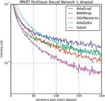
Figure 3. Different optimization methods graph on a Multilayer perceptron training (Retrieved on February 7, 2022, from https://machinelearningmastery.com/adam-optimization-algorithm-for-deep-learning/)
A crucial aspect of ADAM 's competitive performance is that it can solve practical deep learning problems with large datasets and models while having to go through a minimal tuning (Karpathy, 2017), as well as epochs to achieve such results. Although having such good performance, later works have suggested the possibility of lacking the ability of adaptive methods to outperform SGD (Wilson et al., 2017) when measured by their skill to generalize. This is, that the model can display proper adaptation when new pieces of information are added to it (Brownlee 2021) from the same dataset as the original input.
4. Training the network and result analysis
4.1. Lung and Colon Cancer Histopathological Images Dataset
For the present study, the main dataset selected was ‘Lung and Colon Cancer Histopathological Images’, which was used on a model of CNN based on Xception’s algorithm architecture, and tested on different hyperparameters, creating their respective Learning Curves for its analysis. These learning curves represent the performance of the model during its training and validation, in other words, a graph of the model 's learning performance over time.
By watching these graphs, the algorithms can be analyzed during their training and validation process on their dataset respectively, where the plotted lines show how close or far the model’s learning, learning or prediction get from the group of samples in the dataset. The goal is to achieve higher accuracy and low loss, when the graph starts to reach a convergence point (Liu et al., 2020) and stabilizes. The optimizers ADAM, ADAGRAD, SGD+momentum, and SGD+Nesterov were respectively tested in the created model with a dataset of 25000 samples, divided into 60% for the Training Process, 20% for the Validation Process, and 20% for the Testing process.
From these Training and Validation tasks, a series of learning curve charts were made, to obtain a better view and easier understanding (Figure 4) from their Accuracy and Loss values (depicted on the y-axis).
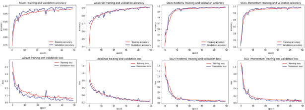
Figure 4. Comparison of learning Curves from Different optimization Algorithms on ‘Lung and Colon Cancer Histopathological Images’ Dataset (from left to right: ADAM, ADAGRAD, SGD+NESTEROV, SGD)
For a fair comparison, the models used the same number of iterations (50 per model) called Epochs (depicted on the x-axis), fed by batches of 32 samples each, and a 180x180 pixels rescaling and tested on a model with different unique Optimizers, which each one presented its advantages and shortcomings.
Also, during these testing and comparison early stages, the models were tested with a Dropout of 0.5 which is the recommended value to start (between 0.2 and 0.5). The dropout value selects the percentage of neurons that is to be discarded during the Validation process, so overspecializing on one aspect is avoided and this creates a bias in its predictions, lowering the accuracy of this model.
This dropout technique is not used during the testing, since all the neurons are used here, that is why the accuracy and loss during the training dataset did not show abrupt peaks as the Validation did.
By randomly discarding leaving inactive a percentage of cells during the Validation process, Dropout helps with generalizing the model and avoids the models entering into a state called overfitting. This is made by allowing the model to focus on the different aspects of the features of input samples, creating a type of impartiality on these features to avoid any predisposition that could affect the judgment of the model predictions.
The results of using different optimizers on one dataset for the recognition of Cancerous Lung cells were brought together. It is clear that Adam works best in matters of overall Accuracy and Loss.
Adam optimizer showed satisfactory results, reaching good accuracy in both the Training and Validation process, and the lack of sudden jumps and drifting suggests that the model graph is slowly reaching into convergence, reaching a minimum Validation Accuracy and Loss of 0.9855 and 0.04 respectively, turning this model into a candidate for further tests with a larger number of Epochs and different Dropout values.
Adagrad optimizer performed well on this Dataset, where it reached early acceptable results, a minimum loss value of 0.1286, and a maximum accuracy of 0.9571, both for the Validation process.
However, their results stagnated on later Epochs, preventing the model from further learning on the current Dataset. As stated before, one of the drawbacks with Adagrad is how it monotonically increases the sum of squares of the gradients on further Epochs, leading to decay of the Learning Rate to decay until the parameter does not update anymore, in other words, it stops learning.
As for ‘SGD + Momentum’, the Learning Curve exhibited relatively slow learning at first, however, it eventually started to improve on a rather stable pattern as it advanced on later Epochs, reaching up to a max accuracy of 0.9744 and min loss value of 0.0876, turning this optimizer version of the model into another candidate for further tests (Zhou et al., 2021), with a larger number of Epochs and a tune of hyperparameters if needed.
Finally, SGD + Nesterov optimization displayed rather stable values, 0.068 for minimum loss and 0.9792 for maximum accuracy, yet not as high as Adam or SGD + Momentum. In this case, the Nesterov optimization method slowed down the learning process preventing the model from both stabilizing and reaching higher accuracy values with a low loss rate.
To corroborate these results, the same optimizers were tested on different datasets, to verify and compare the results with those shown in Figure 4.
4.2. Kather 2016 Dataset
After the training process done on ‘Kather_texture_2016_image_tiles_5000’ Dataset, the results from the learning curves show the performance of the models (Figure 5), all of them with a Dropout value of 0.5, and separated by the Optimizer that was used on it for the current Dataset in batches of 32 samples, alongside with a rescaling of the size of the image down to 180 x 180 pixels.
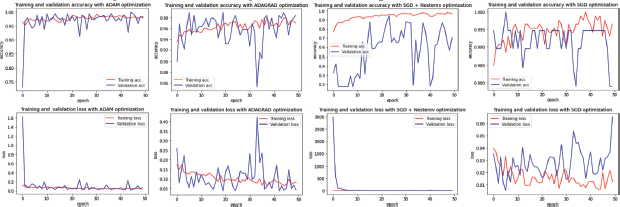
Figure 5. Comparison of learning Curves from Different optimization Algorithms on ‘Kather_texture_2016_image_tiles_5000’ Dataset (from left to right: ADAM, ADAGRAD, SGD+NESTEROV, SGD)
On the current dataset results (Figure 5), through the learning curve is observable that ADAM model was presenting the most stable pattern among all the other optimizers.
As expected, ADAM optimizer showed promising results, similar to those on ‘Lung and Colon Cancer Histopathological Images’ Dataset. In this case, the learning curve for Validation Accuracy showed peaks so high reaching a max 100% accuracy, and an average of 0.968 accuracy during the 50 Epochs, showing a slow tendency to stabilize on every recurrence, without quite finding a convergence point on early Epochs.
On the other hand, on the Learning Curve for Loss Function, it is noticeable how the gaps are relatively small. Moreover, the gaps reach a minimum loss of 0.0135, meaning that the model is prone to avoid making mistakes or incorrect predictions during the testing process, which is paramount during cancer detection, affecting greatly the patient’s diagnosis.
Also, it is noticeable how Adagrad optimizer, despite having peaks sometimes gets closer to an ideal model, does not get to stabilize. However, a good strategy is seizing this optimizer’s skill of reaching higher Accuracy values in early Epochs, in case of encountering learning stagnation problems in later stages. In this case, reaching a minimum loss of 0.0366 and maximum accuracy value of 0.9895 during the Validation process.
On the other hand, ‘SGD + Nesterov’ did not show as good results as those visible on the previous dataset (Figure 4), however, this optimizer´s Loss Learning Curve remained low and stable. These metrics reveal that this model is not suitable yet to fully extract the features of the samples of this dataset properly, although there is a possibility for improvement of the feature extraction by applying different techniques such as data augmentation in the data, to create bigger a sample set that proposes new opportunities to the model, to obtain more features of each class (Dönicke et al., 2019; Candemir et al., 2021) of the dataset.
Nonetheless, this model reached a maximum accuracy value of 0.9474, which although being acceptable, is not as high as the other versions of this model, and a loss value of 0.1351 which is rather high on a metric whose goal is to be as low as possible.
Lastly, the ‘SGD’ optimization method displayed a performance full of peaks on this dataset. The momentum concept allows to minimize the attention that is paid from the model to details, this method helps to avoid overfitting while boosting the learning speed.
At first glance, the gaps on the model, especially those close to the 50th Epoch would tell it’s straying far away from convergence, but this can also be seen as a result of the momentum, which in this case produced positive Accuracy results, having an average of 0.991774, which is impressively high, a maximum Validation Accuracy of 100, and a loss value of 0.0052
4.3. NCT-CRC-HE-100K Dataset
Finally, the results (Figure 6) confirm how the ADAM optimization method was the one who performed the best at the end of the training phase from the ‘NCT-CRC-HE-100K’ Dataset, followed by SGD+Nesterov.
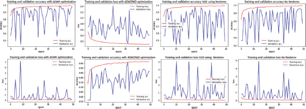
Figure 6. Comparison of learning Curves from Different optimization Algorithms on ‘NCT-CRC-HE-100K’ Dataset (from left to right: ADAM, ADAGRAD, SGD+NESTEROV, SGD)
Similarly, with the other datasets, the parameters used for these models were batches of 32 samples at the time and a rescaling of 180 x 180 pixels, a Dropout value of 0.5, and a Momentum value of 0,9.
By observing the results obtained from this third dataset, and comparing them with those from the other two datasets, it is noticeable how ADAM maintained its great performance, with a maximum Validation Accuracy of 0.9855 and a minimum Loss of 0.0492, outperforming the other optimizers, such as Adagrad model which presented an Accuracy value average of 0.779, except counted times when hitting a maximum Accuracy value of 0.9518 and Loss rate of 0.1286
‘SGD+ Nesterov’ showed a good performance, similar to ‘SGD with Momentum’, both above 97% of Accuracy, and rather low Loss values of 0.0876 and 0.0876 respectively.
After plotting the learning curves from different optimizers, it becomes perceptible how Adam, despite having some peaks, still shows a tendency to a convergence point, displaying a good overall on the different datasets, and for this reason, this optimizer was chosen for further experiments in order to obtain an optimal model with efficient predictions, which is paramount at the moment to detect cancerous cells at early stages saving lives.
The result values during each Training and Validation process are presented in Table 1, divided by each dataset on every tested optimizer, count of how many values during these Epochs did not rise above a threshold of ‘0.1’ for Loss, and those which were able to exceed a value of 0.95.
Table 1. Performance Results and Comparison for Optimizers on custom model on Kather, CRC-VAL-HE-7K, and LC25000 Datasets
|
|
LOSS |
ACC |
VAL LOSS |
VAL ACC |
MIN LOSS |
MAX ACC |
MIN VAL LOSS |
MAX VAL |
AVG ACC |
AVG VAL LOSS |
AVG VAL ACC |
Sum of Speed |
|
ACC |
AVG LOSS |
|||||||||||||
KATHER |
ADAM |
48 |
50 |
39 |
44 |
0.0061 |
0.993 |
0.0135 |
1 |
0.063276 |
0.97764 |
0.103282 |
0.96893 |
1720 |
ADAGRAD |
29 |
47 |
29 |
35 |
0.0624 |
0.9803 |
0.0366 |
0.9895 |
0.102746 |
0.96352 |
0.110252 |
0.958314 |
1720 |
|
SGD+Nesterov |
12 |
27 |
0 |
0 |
0.0638 |
0.9815 |
0.1351 |
0.9474 |
0.174932 |
0.939612 |
79.008334 |
0.561362 |
1576 |
|
SGD |
50 |
50 |
50 |
50 |
0.0063 |
1 |
0.0052 |
1 |
0.016194 |
0.994618 |
0.027376 |
0.991774 |
1733 |
|
ADAM (0.2 Dropout) |
79 |
89 |
19 |
34 |
0.016 |
0.9954 |
0.0228 |
0.9947 |
0.089106 |
0.970348 |
0.679409 |
0.852684 |
9297 |
|
ADAM (0.5 Dropout) |
1 |
30 |
0 |
4 |
0.0945 |
0.9678 |
0.1226 |
0.9575 |
0.172607 |
0.940304 |
0.650614 |
0.8614 |
4303 |
|
CRC-VAL-HE- |
ADAM |
40 |
47 |
4 |
10 |
0.0265 |
0.9913 |
0.0492 |
0.9855 |
0.076972 |
0.972408 |
0.773822 |
0.848666 |
9696 |
ADAGRAD |
10 |
29 |
0 |
1 |
0.0872 |
0.9718 |
0.1286 |
0.9571 |
0.154862 |
0.939204 |
0.629188 |
0.77994 |
] 8158 |
|
ADAM 0.2 DROPOUT |
90 |
96 |
15 |
26 |
0.0061 |
0.9981 |
0.0072 |
0.9965 |
0.05107 |
0.981726 |
0.923743 |
0.839584 |
17947 |
|
ADAM (0.5 Dropout) |
100 |
100 |
31 |
51 |
0.0127 |
0.9969 |
0.0191 |
0.9947 |
0.04181 |
0.9862 |
0.42132 |
0.928086 |
6501 |
|
SGD+MOMENTUM |
41 |
45 |
2 |
2 |
0.0154 |
0.9941 |
0.0876 |
0.9744 |
0.071768 |
0.97306 |
1.127848 |
0.752724 |
7800 |
|
LC25000 |
ADAM |
40 |
47 |
4 |
10 |
0.0265 |
0.9913 |
0.0492 |
0.9855 |
0.076972 |
0.972408 |
0.773822 |
0.848666 |
9696 |
ADAGRAD |
10 |
29 |
0 |
1 |
0.0872 |
0.9718 |
0.1286 |
0.9571 |
0.154862 |
0.939204 |
0.629188 |
0.77994 |
1720 |
|
SGD+Nesterov |
41 |
45 |
2 |
5 |
0.0238 |
0.9913 |
0.068 |
0.9792 |
0.079746 |
0.970302 |
0.80578 |
0.807776 |
1576 |
|
SGD |
41 |
45 |
2 |
2 |
0.0154 |
0.9941 |
0.0876 |
0.9744 |
0.071768 |
0.97306 |
1.127848 |
0.752724 |
1733 |
|
ADAM (0.2 Dropout) |
90 |
96 |
15 |
26 |
0.0061 |
0.9981 |
0.0072 |
0.9965 |
0.05107 |
0.981726 |
0.923743 |
0.839584 |
9297 |
|
ADAM (0.5 Dropout) |
88 |
96 |
15 |
27 |
0.0074 |
0.9971 |
0.0434 |
0.9841 |
0.052853 |
0.98102 |
0.46387 |
0.889964 |
4303 |
|
Table 1 also displays the Maximum Accuracy and Minimum Loss value that each model reached during its Validation, followed by an overall average of Accuracy and Loss for a better understanding of this model behavior towards the selected Dataset, and lastly, the time required (measured in seconds) to complete the whole process.
These experimental results summarized in Table 1 provide a comparison between optimizers on the proposed classification method on different datasets, where so is observable the improvement between each Optimizer on the current Model, delivering initial results on the projected classification pipeline.
Overall, the model achieved on its performance a peak of 99.8% and 99,7 of accuracy on Adam with 0.2 Dropout and 0.5 Dropout respectively and a loss of 0.006% and 0.0074%. The overall result displayed by the proposed model is able to capture features from cell slides to detect cancerous cells in patients in real-world scene scenarios.
From the table, it was evident which models performed the best, and by diagnosing the properties of their Learning curves, the datasets can be analyzed as well as the model behavior during the fitting process. In this case, sudden jumps and drops shown on the Learning Curves suggest that the validation dataset is unrepresentative
4.4. Unrepresentative Dataset
This definition applies to datasets with a small number of samples compared to a large, representative dataset. Resulting in poor feature extraction by the model that is in training, thus a low accuracy and high error rate on our model, regardless of the quality of it.
In the field of Deep Learning, the use of a high-quality model and a good optimizer alone is not enough to achieve satisfactory results. Nevertheless, the dataset that is employed is a paramount factor for accomplishing the desired outcome.
When choosing a Dataset, there are several factors to have in mind, such as the presence or lack of noise from the samples, and mostly the availability of the data, whether be due to rather scarce data or the lack of public information in existence. The analysis of a problem of this nature has a big impact on choosing an optimal size of samples needed to feed the model. There is no concise number of samples for a perfect sized dataset, since it varies depending on the nature and complexity of the problem, or on the level of robustness of the model at hand. Nevertheless, an answer which fits is likely an impossible task, but it is advised to start from the factor 10 rule for sample size requirements, which means to have a number of samples at least 10 times more (Alwosheel et al., 2018) than the number of parameters.
Even by following the factor 10 rule, the optimal size of samples for the selected dataset might not be achieved. In occasions where the difference between classes is small, a larger selection might be necessary, as for example to work with ImageNet Dataset database (Deng et al., 2009), it is recommended at least 1000 examples per class (Krizhevsky et al., 2012) for training data.
An optimal dataset selection allows the network to achieve a better generalization, which is observable after the model has concluded the training and validation process. The two most common cases that could arise during the fitting process are Unrepresentative Training Dataset, and Unrepresentative Validation Dataset.
4.5. Unrepresentative Training Dataset
The training dataset lacks sufficient information to facilitate learning compared to the validation dataset, which prevents a learner or model from achieving high accuracy and a smaller loss rate.
This situation can be easily identified by a learning curve of training loss that shows improvement and similarly to the learning curve for validation loss that also shows improvement, but a large gap remains between both curves (Figure 7).
Figure 7. Unrepresentative Training Dataset Learning Curve
Even after applying the factor’ 10 rule, when the sample size is too small, a display of rather noisy results on the Learning Curve is obtained, exhibiting a visible inconsistency between train and validation outcome. In such cases, an alternative is to re-do a split of the data samples with the idea that the new examples may be more significant and representative of the model at the moment of extracting its features, as well as applying data augmentation techniques to improve the quality and quantity of the samples provided to the Training Dataset.
4.6. Unrepresentative Validation Dataset
This case occurs when it is not possible to evaluate the generalization ability of the model from the validation dataset, which is to say when there are too many examples from the validation dataset in contrast with the training dataset. This can be observed in a learning curve that appears to fit the training loss well (or other fitting curves) and a learning curve that appears to fit the validation loss well but is characterized by noise. On the learning curves from Loss training, excellent results seem to appear evident, and yet, show unstable changes as is observable on sudden high and low peaks on the validation loss (Figure 8).
Figure 8. Unrepresentative validation dataset
In this second example is noticeable the same jumps and drops as those from the learning curve in the model of study, since during the training the data was rather limited and after using different techniques such as Data Augmentation for increasing the number of samples, the validation data was still unrepresentative compared to the training data.
This model’s training was made on a Dropout of 0.5, this means that during the training process (it does not use this during the validation process) 50% of features nodes or neurons are set to 0 because they are not going to be used.
Dropout helps with generalizing the model and avoids the models enter into a state called overfitting.
This dropout technique is not used during the testing, since here all the neurons are used, that is why the accuracy and loss during the dataset training did not show abrupt peaks as the Validation did.
After performing this exploratory testing on Lung Cancer Database, using different Hyperparameters on the best performing optimizer so far (ADAM), the input values for these Dropouts were 0.5 and 0.2 respectively, which after plotting the learning curve, produced similar results, after a larger number of Epochs (Figure 9, Figure 10).
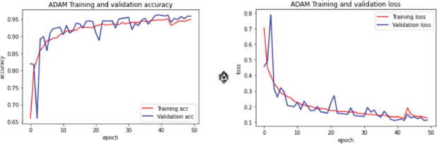
Figure 9. Learning Curve for ADAM optimization with 0.5 Dropout
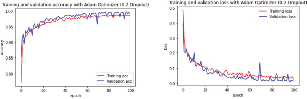
Figure 10. Learning Curve for ADAM optimization with 0.2 Dropout
In the current study case (Figure 10) the learning curves showed how a higher Dropout of 0.5 resulted in a rather stable Validation Loss in comparison with 0.2, which makes sense as the model by discarding half of the neurons allow itself to avoid wrong weights or paths easier, but this also has affected the Validation Accuracy where a lower dropout value of 0.2 (Figure 10) exposed better results on validation accuracy, which is acceptable in this model since it got a positive outcome during the evaluation of this model, delivering a Validation Accuracy of 0.9965 and a Validation loss of 0.0072.
Thus, in this study case, the chosen optimizer for this model was Adam on a Dropout of 0.2 since the overall proved to be better as its observable while transposing the learning curve results as it’s shown on Figure 11.
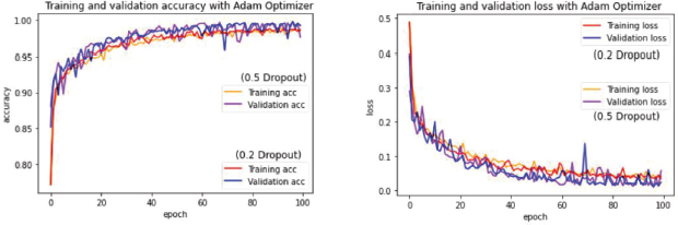
Figure 11. Juxtaposition of learning rates from different Dropout values on ADAM optimization method
Other studies suggest the possibility a different approach of SGD actually outperforming ADAM in later stages or epochs during the training of the model by Switching from ADAM to SGD (SWATS).
This strategy was tested in cases such as Tiny-ImageNet problem, where the switches from Adam to SGD lead to significant though temporary degradation in their performance. This is, after an abrupt drop from 80% to 52% caused by this switch, the model eventually recovered, achieving an even better peak on testing accuracy compared to Adam, which in some cases lead to a stagnation (Keskar and Socher, 2017) in performance.
5. Results of the final model
Once the best model was chosen from the training made on our model, the next step was to set a Classification Report (Figure 12) as well as a Confusion Matrix (Figure 13) to measure its performance, showing on the center the accurate predictions it made on the dataset.
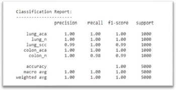
Figure 12. Classification Report of Model Performance
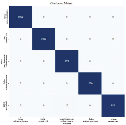
Figure 13. Confusion Matrix from final model on selected optimizer (Adam)
6. Conclusions
In this research, several methods for improving the model’s classification performance were proposed, testing them and proving their effectiveness on the selected datasets. The result of this study saves exploration time when creating new models for cancer detection, as well as getting better performance in practical applications in real life.
The purpose of this research was to test various optimizers namely Adagrad, Adam, SGD + Momentum, and SGD + Nesterov.
While Adam, SGD + Momentum, and SGD + Nesterov optimizers took their time to achieve good values for Accuracy and Loss, Adagrad obtained good results on early epochs but reached stagnation during some sessions, which could be problematic when working with more classes on larger training periods.
‘SGD+Nesterov’ showed really good results, yet on scarce occasions, as with ‘SGD+Momentum’ which also achieved great results, except for those on Kather Dataset (Figure 5).
Finally, and after these experiments, Adam optimizer was selected for having the best performance during the training and validation process, being the one which obtained the best results during this cancer-classification task as it was explained in the Network Training and Result Analysis section.
From the Confusion Matrix (Figure 13), it becomes evident why Adam proved to be the right choice, as the diagonal values of this Matrix show a high rate of accurate prediction hits on each of these 5 classes achieving a perfect score of 1000 right guesses from 1000 samples for 3 of the selected classes(Lung Adenocarcinoma, Lung Normal cell, and Colon Adenocarcinoma).
On the rows arranged next to the principal diagonal of this Matrix, are the wrong predictions which did not match with the actual class, yet remaining competitive results with 999 right guesses on Lung Squamous Cell Carcinoma class, and 985 correct predictions from Lung Squamous Cell Carcinoma class, this last one being the lowest between the 5 classes.
The use of Deep Learning on medical fields such as Cancer recognition models have many challenges; since every cell is different and cancer works randomly on cells, the use of techniques to improve the input data allows to overcome these obstacles, reaching higher accuracy values as well as a better generalization ability. Still, the algorithm proposed on the current study has shown promising features, such as high precision and low loss rate, runs relatively fast, combining different techniques and approaches as a deep learning algorithm.
With the aim of solving the problems of low detection accuracy of cancerous targets, the use of Depthwise Separable Convolutions was selected for this CNN model, since its architecture has fewer parameters than those on commonly used, thus is less prone to overfitting.
Although the accuracy of cancer detection has improved to a certain extent, further studies must be carried out to improve and perfect these models and techniques to achieve better and optimal results on this task. The success of this research motivates future in-depth exploration of the dynamics, with different optimizer and generalization in later epochs where the optimal convergence is harder to reach.
References
Alwosheel, A., van Cranenburgh, S., and Chorus, C. G., 2018. Is your dataset big enough? Sample size requirements when using artificial neural networks for discrete choice analysis. Journal of Choice Modelling, 28, 167–182. 10.1016/j.jocm.2018.07.002.
Alzubaidi, L., Zhang, J., Humaidi, A.J., et al., 2021. Review of deep learning: concepts, CNN architectures, challenges, applications, future directions. J Big Data 8, 53. https://doi.org/10.1186/s40537-021-00444-8.
Bengio, Y., Courville, A., and Vincent, P., 2014. Representation Learning: A Review and New Perspectives. [cs.LG]. Opgehaal van http://arxiv.org/abs/1206.5538.
Bengio, Y., 2012. Practical Recommendations for Gradient-Based Training of Deep Architectures. Neural Networks: Tricks of the Trade.
Brownlee, J., 2021. Gentle Introduction to the Adam Optimization Algorithm for Deep Learning. Machine Learning Mastery. Retrieved February 7, 2022, from https://machinelearningmastery.com/adam-optimization-algorithm-for-deep-learning/.
Borkowski A. A., Bui M. M., Thomas L. B., Wilson C. P., DeLand L. A., and Mastorides S. M., 2019. Lung and Colon Cancer Histopathological Image Dataset (LC25000). https://doi.org/10.48550/arXiv.1912.12142 [eess.IV].
Candemir, S., Nguyen, X. V., Folio, L. R., and Prevedello, L. M., 2021. Training Strategies for Radiology Deep Learning Models in Data-limited Scenarios. Radiology: Artificial Intelligence, 3(6), e210014. https://doi.org/10.1148/ryai.2021210014.
Chan, H. P., Hadjiiski, L. M., and Samala, R. K., 2020. Computer-aided diagnosis in the era of deep learning. Medical physics, 47(5), e218–e227. https://doi.org/10.1002/mp.13764) (Sarah J. MacEachern and Nils D. Forkert. Machine learning for precision medicine. Genome. 64(4): 416–425. https://doi.org/10.1139/gen-2020-0131.
Cheng, J., Benjamin, A., Lansdell, B., and Kordin, K. P., 2021. Augmenting Supervised Learning by Meta-learning Unsupervised Local Rules. CoRR, abs/2103.10252. Opgehaal van https://arxiv.org/abs/2103.10252.
Deng, J., Dong, W., Socher, R., Li, L. J., Li, K., and Fei-Fei, L., 2009. ImageNet: A large-scale hierarchical image database. 2009 IEEE Conference on Computer Vision and Pattern Recognition, 248–255. https://doi.org/10.1109/CVPR.2009.5206848.
Dönicke, T., Lux, F., and Damaschk, M., 2019. Multiclass Text Classification on Unbalanced, Sparse and Noisy Data.
Elashmawi, H., 2019. «Optimization of Mathematical Functions Using Gradient Descent Based Algorithms». Mathematics Theses. 4. https://opus.govst.edu/theses_math/4.
Gylberth, R., 2018. Momentum Method and Nesterov Accelerated Gradient - Konvergen. AI. Medium. Retrieved February 6, 2022, from https://medium.com/konvergen/momentum-method-and-nesterov-accelerated-gradient-487ba776c987.
Hirsch, F. R., Franklin, W. A., Gazdar, A. F., and Bunn, P. A., 2001. Early Detection of Lung Cancer: Clinical Perspectives of Recent Advances in Biology and Radiology. Clinical Cancer Research, 7(1), 5–22. Opgehaal van https://clincancerres.aacrjournals.org/content/7/1/5.
Hussain Z., Gimenez F., Yi D., and Rubin D., 2017. Differential Data Augmentation Techniques for Medical Imaging Classification Tasks. AMIA. Annual Symposium proceedings. AMIA Symposium. 2017:979–984. PMID: 29854165; PMCID: PMC5977656.
Johnson, K. B., Wei, W. Q., Weeraratne, D., Frisse, M. E., Misulis, K., Rhee, K., Zhao, J., and Snowdon, J. L., 2021. Precision Medicine, AI, and the Future of Personalized Health Care. Clinical and translational science, 14(1), 86–93. https://doi.org/10.1111/cts.12884.
Karpathy, A., 2017. A Peek at Trends in Machine Learning. https://karpathy.medium.com/a-peek-at-trends-in-machine-learning-ab8a1085a106. [Online; accessed 12-Dec-2017].
Kather, J. N., Halama, N., and Marx, A., 2018. 100,000 histological images of human colorectal cancer and healthy tissue (v0.1).
Kather J. N., Weis C. A. , Bianconi F., Melchers S. M., Schad L. R., Gaiser T., Marx A., and Zollner F., 2016. Multi-class texture analysis in colorectal cancer histology. Scientific Reports (in press).
Keskar, N., and Socher, R., 2017. Improving Generalization Performance by Switching from Adam to SGD. https://doi.org/10.48550/arXiv.1712.07628.
Kingma, D. P., and Ba, J., 2015. Adam: A Method for Stochastic Optimization. CoRR. https://doi.org/10.48550/arXiv.1412.6980
Krizhevsky, A., Sutskever, I., and Hinton, G. E., 2012. ImageNet Classification with Deep Convolutional Neural Networks. In F. Pereira, C. J. C. Burges, L. Bottou, and K. Q. Weinberger (Reds), Advances in Neural Information Processing Systems (Vol 25). Opgehaal van https://proceedings.neurips.cc/paper/2012/file/c399862d3b9d6b76c8436e924a68c45b-Paper.pdf.
Liu, Z., Xu, Z., Rajaa, S., Madadi, M., Junior, J. C. S. J., Escalera, S., Pavao, A., Treguer, S., Tu, W., and Guyon, I., 2020. Towards Automated Deep Learning: Analysis of the AutoDL challenge series 2019. Proceedings of the NeurIPS 2019 Competition and Demonstration Track, in Proceedings of Machine Learning Research. Available from https://proceedings.mlr.press/v123/liu20a.html.
More, A., 2016. Survey of resampling techniques for improving classification performance in unbalanced datasets. [stat.AP]. Opgehaal van http://arxiv.org/abs/1608.06048.
Najafabadi, M. M., Villanustre, F., Khoshgoftaar, T. M., et al., 2015. Deep learning applications and challenges in big data analytics. Journal of Big Data 2, 1. https://doi.org/10.1186/s40537-014-0007-7.
Ozawa, T., Ishihara, S., Fujishiro, M., Kumagai, Y., Shichijo, S., and Tada, T., 2020. Automated endoscopic detection and classification of colorectal polyps using convolutional neural networks. Therapeutic advances in gastroenterology, 13, 1756284820910659. https://doi.org/10.1177/1756284820910659.
Ruder, S., 2016. An overview of gradient descent optimization algorithms, pp. 11. https://doi.org/10.48550/arXiv.1609.04747.
Schmidt, D., 2018. Understanding Nesterov Momentum (NAG). https://dominikschmidt.xyz/nesterov-momentum/
Scholte, M., van Dulmen, S. A., Neeleman-Van der Steen, C. W. M., et al., 2016. Data extraction from electronic health records (EHRs) for quality measurement of the physical therapy process: comparison between EHR data and survey data. BMC Med Inform Decis Mak 16, 141. https://doi.org/10.1186/s12911-016-0382-4.
Shorten, C., and Khoshgoftaar, T. M., 2019. A survey on Image Data Augmentation for Deep Learning. J Big Data 6, 60. https://doi.org/10.1186/s40537-019-0197-0
Sutskever, I., Martens, J., Dahl, G., and Hinton, G., 2013. On the importance of initialization and momentum in deep learning. Proceedings of the 30th International Conference on Machine Learning, in PMLR- 28(3):1139–1147.
Taghiakbari, M., Mori, Y., and von Renteln, D., 2021. Artificial intelligence-assisted colonoscopy: A review of current state of practice and research. World journal of gastroenterology, 27(47), 8103–8122. https://doi.org/10.3748/wjg.v27.i47.8103.
Tom, J., Fei-Fei, L., Ranjay, K., Leila, A., Amil, K., and Chen, C. K., 2020. CS231n: Convolutional Neural Networks for Visual Recognition. https://cs231n.github.io/neural-networks-3/.2020.
Wilson, A., Roelofs, R., Stern, M., Srebro, N., and Recht, B., 2017. The Marginal Value of Adaptive Gradient Methods in Machine Learning. NIPS.
Xue Y., Chen S., Qin J., Liu Y., Huang B., and Chen H., 2017. Application of Deep Learning in Automated Analysis of Molecular Images in Cancer: A Survey. Contrast Media & Molecular Imaging, vol. 2017, Article ID 9512370, 10. https://doi.org/10.1155/2017/9512370.
Ye, G. B., and Xie, X., 2012. Learning sparse gradients for variable selection and dimension reduction. Mach Learn 87, 303–355. https://doi.org/10.1007/s10994-012-5284-9.
Zhou, B. C., Han, C. Y., and Guo, T. D., 2021. Convergence of Stochastic Gradient Descent in Deep Neural Network. Acta Math. Appl. Sin. Engl. Ser. 37, 126–136. https://doi.org/10.1007/s10255-021-0991-2.
Zhou, P., Feng, J., Ma, C., Xiong, C., Hoi, S., and Weinan, E., 2020. Towards Theoretically Understanding Why SGD Generalizes Better Than ADAM in Deep Learning. https://doi.org/10.48550/arXiv.2010.05627.
Authors’s Biography

David Zambrano, received a Master Degree in Computer Science and Technology from Harbin University of Science and Technology, located in Harbin, China, in 2022. Following my vocation and Life Project, been working with technology on world of education for 7 years, and research about technological advances such as Deep Learning Besides technology, my interests reside on languages, currently learning Chinese as my fifth language, focusing on taking advantage of languages, such as for obtaining information all around the world, for researching and creating solutions on benefit of society.

Sun Bowen, University of Science and Technology and a master tutor in computer science and technology. In 1999, he founded the «Fractal Channel» website. Two sets of «Internet Times» programs of CCTV were broadcasted on February 27, 2002 to introduce the «Fractal Channel» website. Sun Bowen ‘s fractal art works have been exhibited in Tianjin Science and Technology Museum, Heilongjiang Science and Technology Museum and other units many times. Research direction: fractal graphics, the complexity of financial markets.