
Regular Issue, Vol. 11 N. 2 (2022), 191-206
eISSN: 2255-2863
DOI: https://doi.org/10.14201/adcaij.27393
|
ADCAIJ: Advances in Distributed Computing and Artificial Intelligence Journal
Regular Issue, Vol. 11 N. 2 (2022), 191-206 eISSN: 2255-2863 DOI: https://doi.org/10.14201/adcaij.27393 |
Deep Learning Approach to Technician Routing and Scheduling Problem
Engin Pekel
Hitit University, Turkey
enginpekel@hitit.edu.tr
ABSTRACT
This paper proposes a hybrid algorithm including the Adam algorithm and body change operator (BCO). Feasible solutions to technician routing and scheduling problems (TRSP) are investigated by performing deep learning based on the Adam algorithm and the hybridization of Adam-BCO. TRSP is a problem where all tasks are routed, and technicians are scheduled. In the deep learning method based on the Adam algorithm and Adam-BCO algorithm, the weights of the network are updated, and these weights are evaluated as Greedy approach, and routing and scheduling are performed. The performance of the Adam-BCO algorithm is experimentally compared with the Adam and BCO algorithm by solving the TRSP on the instances developed from the literature. The numerical results evidence that Adam-BCO offers faster and better solutions considering Adam and BCO algorithm. The average solution time increases from 0.14 minutes to 4.03 minutes, but in return, Gap decreases from 9.99% to 5.71%. The hybridization of both algorithms through deep learning provides an effective and feasible solution, as evidenced by the results.
KEYWORDS
Adam algorithm; deep learning; optimization; technician routing and scheduling
1. Introduction
Optimized systems are one of the keys to success in today's competitive world. This situation is encountered in almost every field. The technician routing and scheduling problem (TRSP) is one of these areas. TRSP can be considered a special case of vehicle routing problems (Pekel and Kara, 2019). TRSP does not only consist of assigning technicians to teams but also of assigning teams to tasks and creating routes. In addition, the selected technician group must meet a certain level of qualification (Pekel, 2020; Zamorano and Stolletz, 2017). In many technician planning problems, routing complexity is crucial. Routing is carried out so that the expert technician group leaves and returns to the central warehouse at the end of the day. Travelling times between each node are computed as Euclidean distance (Khalfay et al., 2017).
The TRSP includes a pre-determined set of technicians who have various talents and a set of tasks requested by the customer at various locations. To perform tasks consisting of customer requests, the set of technicians is divided into teams, and teams travelling in different locations are assigned the tasks. When teams are assigned tasks, the constraint of compatibility between tasks requiring different skills and teams of technicians with different skills is considered. Time windows are defined for the tasks requested by the customer, and requests must be fulfilled during these time intervals. Besides, technicians perform tasks for a specific period, and overtime occurs when this time interval is exceeded. Once and for all, the service times of the tasks, travel times, and the skill requirements required for each task are known in advance.
Algorithms have been developed to provide many exact solutions to TRSP so far in the literature. Charris et al. (2019) implemented a decision support system to optimise technicians' routes in Colombia. In their work, technicians performed daily tasks received from customers. Mathlouthi et al. (2018) maximized the maintenance and repair of electronic process equipment by subtracting total profit from operating costs. Anoshkina and Meisel (2019) tackled the issue of combined teams of workers and routes while considering costs. Chen et al. (2016) presented the technician orientation model that creates experience-based learning, aiming to minimize the time taken to fulfil the final task. The authors used the heuristic method of travel from record to record (RTR) in solving the model. Kovacs et al. (2012) consider technicians with several skills at several levels grouped into teams to fulfil routing decisions and upkeep tasks and establish the Service TRSP. Pekel (2020) suggested an improved PSO (IPSO) algorithm to solve TRSP using a specific dataset. Graf (2020) considered a multi-period vehicle and technician routing and scheduling problem and proposed a combination of large neighbourhood and local search heuristics and a decomposition approach to efficiently generate competitive solutions under restricted computational resources. The authors’ numerical results showed that the method is efficient and effective, especially under tight time restrictions. Çakırgil et al. (2020) dealt with multi-skilled workforce scheduling and routing problem in field service operations motivated by a daily, real-life problem faced by electricity distribution companies. They proposed a two-stage matheuristic to obtain a good approximation of the Pareto frontier since the computational effort considerably increases in real-life problem instances. Mathlouthi et al. (2021) dealt with technician routing and scheduling problems motivated by an application to repair and maintain electronic transactions equipment. The problem exhibits many special features, such as multiple time windows for service, a spare parts inventory taken by each technician, and tasks that may require a special part to be performed. The authors used a methodology based on Tabu search, coupled with an adaptive memory.
Deep learning first entered our lives mainly in the form of forecasting and clustering, but nowadays, it is beginning to be used effectively in combinational optimization problems. Fu et al. (2020) investigated vehicular energy networks' stability and efficiency to optimize the routing and dynamic storage allocation of renewable energy by integrating a time-expanded topology graph and a deep learning method. Authors applied deep learning to improve the prediction accuracy of the traffic pattern. Wang and Sun (2020) proposed a multi-agent deep reinforcement learning method to develop a bus route that is dynamic and has flexible holding control strategies. The authors used a headway-based reward function to train their proposed method. Hussain et al. (2021) researched the progress of machine learning in vehicle networks for intelligent route decisions. Lee et al. (2020) proposed a route and charging station algorithm based on a model-free deep reinforcement learning method to deal with the uncertainty of traffic conditions by minimizing the total travel time. James et al. (2019) proposed a novel deep reinforcement learning-based neural combinatorial optimization strategy. The authors used a deep reinforcement learning mechanism with an unsupervised auxiliary network to train the model's parameters. Koh et al. (2020) proposed a deep reinforcement learning method to construct a real-time intelligent vehicle routing and navigation system. Also, the authors used intelligent agents to facilitate intelligent vehicle navigation. Hernández-Jiménez et al. (2019) explored a deep learning approach to the routing problem in vehicular delay-tolerant networks by performing a routing architecture and deep neural networks.
The paper's main contributions are as follows: a combinational optimization problem is solved by performing deep learning in TRSP for the very first time. Also, the Adam algorithm is integrated with the BCO method and obtains decent and fast solutions.
The remainder of the article is organised as follows: Section 2 describes the model of TRSP. Section 3 presents the method that consists of the Adam algorithm, Body change operator (BCO) and the Adam-BCO method. Section 4 offers the numerical results of the algorithms for Pekel's benchmark instances. Finally, Section 5 outlines all the findings and draws conclusions from them.
2. Mathematical Model
This paper does not propose an algorithm to provide an exact solution, however, the mathematical model of the problem is presented. I represents one central depot and tasks. TRSP consists of arcs, K teams, D days, days allowed to visit a task, I tasks, M technicians, L proficiency levels, and Q skills. A generated technician team visits from node i to node j, considering cij visiting cost and pi service time of node i. Visiting operation must be completed within the earliest aid and the latest bid bid, considering daily work hours [e,f]. Started works cannot be interrupted. The generated technician team has δ number of technicians, and this paper chooses δ = 2. The mathematical model accepts different values for δ if requested. When the number of technicians was more than 2, there was a slight increase in the time the model required to obtain the solution, and more straightforward solutions were obtained. Each task requires vid : {0or 1} proficiency, and each technician has proficiency level gmg : {0or 1}. The model allows ωcost cost of waiting time and otcost cost of overtime. However, this paper does not allow ωcost and otcost. All sets and parameters are described above. Table 1 shows the decision variables of the model.
Table 1. Notation
Decision variables |
|
Xijkd |
1 if team k fulfills task i and visits task j on day d, 0 otherwise |
Yijk |
1 if team k carries out task i on day d, 0 otherwise |
Zmkd |
1 if technician m works for team k on day d, 0 otherwise |
Sijk |
Beginning time of the task i carried on team kand day d |
ωi |
Staying time of task i |
otkd |
Overtime of team k on day d |
12\* MERGEFORMAT ()
34\* MERGEFORMAT ()
56\* MERGEFORMAT ()
78\* MERGEFORMAT ()
910\* MERGEFORMAT ()
1112\* MERGEFORMAT ()
1314\* MERGEFORMAT ()
1516\* MERGEFORMAT ()
1718\* MERGEFORMAT ()
1920\* MERGEFORMAT ()
2122\* MERGEFORMAT ()
2324\* MERGEFORMAT ()
2526\* MERGEFORMAT ()
2728\* MERGEFORMAT ()
2930\* MERGEFORMAT ()
3132\* MERGEFORMAT ()
3334\* MERGEFORMAT ()
3536\* MERGEFORMAT ()
Equation (1) is the model's objective function and minimizes the total travelling cost. ωcost and otcost are equal to zero since this paper does not allow waiting time and overtime. Equations (2) and (3) guarantee that each task is visited in the planned time windows. Each generated team completes its routed tasks starting and ending from the same central depot in equations (4) and (5). At least one team must be created for each day. Equation (6) provides the flow of tasks in a team and day. Equation (7) both avoids sub-tours and calculates the starting times of tasks. Equations (7) - (9) enable the tasks to start and end according to their time windows. Equations (7) - (11) are non-linear limitations. However, constraints are linearized by a big M formulation (7) - (11). The transformation of the 7th and 8th equations into linear format with Big M is shown in equations (19) and (20). The remaining equations (9) – (11) were made linear in the same way.
3738\* MERGEFORMAT ()
3940\* MERGEFORMAT ()
Equations (10) and (11) enable the tasks to start and finish according to daily working hours. When starting the route for the first task from the depot, the starting time is assumed to be greater than or equal to max{e, aid}. Equation (12) impedes the inclusion of a technician in more than one team per day, and Equation (13) ensures that the number of technicians in the teams is equal to the predetermined value. Equation (14) guarantees that the skills of the chosen technicians satisfy the mastery essentials for the routed tasks. Equations (15) and (16) provide lower and upper bounds to waiting time and overtime, respectively. Equation (17) ensures that the starting time is a positive variable, and constraint (18) defines the specified variables as binary.
Figure 1 shows the illustration of the mathematical model for TRSP.
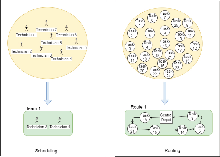
Figure 1. An illustration of the mathematical mode
3. Methodology
The methodology section describes the three different methods applied in this study. These methods are the Adam algorithm, the BCO method, and the Adam-BCO hybrid algorithm. Also, the network structure of the algorithms applied in this section is provided.
There are 26 hidden neurons in the first hidden layer. The main reason for choosing 26 neurons is that there are 25 customers and one central depot in the discussed TRSP. Since there are 26 nodes, 26 neuron and input entries are made. Two hidden layers are used in the network structure. Applications have been made to use more than two hidden layers, but practical results have not been obtained. The connections between the inputs and hidden neurons in the first layer are considered arc connections. Adam and Adam-BCO hybrid algorithms train arc connections, taking the maximum weight value. The maximum weight value passes through the arc connections on the second and first hidden layers, and the maximum weight is selected as the Greedy rule. If the obtained route meets the feasibility conditions, deep learning provides a new routing and the technician groups' scheduling.
Figure 2 shows the network structure of deep learning implemented in TRSP. For example, let's assume that there is an assignment from task 8 to complete task 1. Let's express this with X [8, 1] = 1. It is checked that this assignment is feasible, and according to a function value created on the basis of the main algorithm, X [8, 1] assignment value can be 0. Thus, new solution spaces are tried.

Figure 2. Deep learning network structure implemented in TRSP
3.1. Adam Algorithm
The ADAM algorithm can be defined as the realization of an efficient stochastic optimization method with only the first-order derivative of the selected function and with minimal memory requirement. The name Adam is derived from adaptive moment estimation and is designed to combine the advantages of the two methods, AdaGrad (Duchi et al., 2011) and RMSProp (Tieleman and Hinton, 2012). The algorithm calculates adaptive learning rates from the outputs of the first and second moments of the gradients, considering the parameters it contains in its structure. The Adam algorithm is an algorithm that includes the advantageous aspects of the RMSProp and momentum methods. It caches the momentum changes as well as the learning rates of each of the parameters; it combines RMSProp and momentum. This provides higher performance in terms of speed.
The obtained learning rates are used to reach the bias-corrected version of the exponential moving averages (Kingma and Ba, 2014). With bias-corrected values, the weights or connection values of the network used for estimation are updated, and it is indented to obtain convergence over the determined iterations or convergence limit. Algorithm 1 shows the mechanism of the Adam algorithm used in TRSP. For the Adam algorithm to work, alpha and two different beta parameters must be determined.
Algorithm 1. Pseudo-code Adam algorithm
Require: α: Step size, β1 and β2 decay rates for the moment estimates
Require: f(θ): Weight of deep-learning with parameters θ
Require: θ0: Initial weights of deep-learning and set to 0
m0 ← 0
ϑ0 ← 0
t ← 0 (Iteration (150))
while currentiteration < t do
t←t+1
: Greedy rule
get the values of gradients (g(θt))
update first-moment estimate (mt)
update second-moment estimate (ϑt)
compute bias-corrected first-moment estimâte (mt)
compute bias-corrected second-moment estimâte (ϑt)
update weights (θt)
end while
return θt
Here, different combinations should be examined while determining their parameters. Within the scope of this study, research was conducted on different parameter values by trial-and-error method and chosen α = 0.0001, β1 = 0.8, and β2 = 0.99. In this paper, inputs refer to actions. Visiting from a node to a different node is considered an action. There are 26 hidden neurons in the first and second hidden layers. The first and second-moment estimate values must be updated for the algorithm to update the net weights. The first-moment estimate is updated with equation mt = β1 * mt-1 + (1 - β1) * gt and the second-moment estimate is updated with equation is the gradient of the tanh function and computed by . Bias is corrected first, and second-moment estimates are computed by , respectively. After updating all the necessary parameters, the weights of the net on the first hidden layer are calculated by . Here, ε = 10−8.
As a result of the calculations, the values of the networks between actions and neurons in the first hidden layer, are obtained. The maximum θt value coming to any hidden neuron in the first hidden layer from the twenty-six inputs, is taken. All the steps described earlier are repeated by taking the value. The network weights (θt) are updated, from the hidden neurons in the second hidden layer to the output neuron. Updated weights allow new routing to be created on the basis of the Greedy rule. While using a Greedy rule-based action selection mechanism, the routing and technician selections to be created should be feasible. To this end, environment simulation is applied while choosing an action.
Figure 3 shows the operation mechanism of the Adam algorithm used to find possible routings and scheduling. Feasible routing and scheduling are done with random data generation. The data created here reveals actions (from one node to the other). (26×26) actions are expressed as the weight value of the network. The weights of the network are updated with the Adam algorithm. Later the update process, the routing, and scheduling process is completed by simulating the environment to verify feasibility.
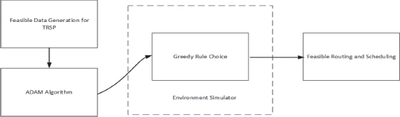
Figure 3. Operation mechanism of Adam algorithm in TRSP
3.2. Body Change Operator
The genetic algorithm is a stochastic solution generation algorithm inspired by the evolutionary process of living things. The development and characteristics of living things are found on chromosomes. The genetic algorithm uses a simple chromosome-like data structure to follow the characteristics of the solution through this structure. The replacement of these structures is provided by mechanisms such as crossing. The variety of problems in which genetic algorithms are applied is quite wide, and genetic algorithms are often seen as the optimizers of the obtained solutions (Whitley, 1994).
The body change operator (BCO) is a solution improvement operator based on a genetic algorithm (Pekel and Kara, 2019). The part where it differs from the genetic algorithm is the absence of mutation. Cross-over operation is performed by crossing sub-routing in a feasible routing, but there is no cross-over ratio. In short, this operator, which makes an improvement process for each solution, works. Algorithm 2 shows the mechanism of the body change operator used in TRSP.
Algorithm 2. Pseudocode of BCO
Initialize: Each chromosome (n: Population size (300))
chp ← 0 (Chromosome position)
chc ← 0 (Chromosome cost)
Gchp ← 0 (Chromosome global position)
Gchc (Chromosome global cost)
t ← 0 (iteration (1))
while currentiteration < t do
perform: Body change operator
compute: Cost function
decide: chc < Gchc
Gchp ← chp
Gchc ← chc
end while
return
The body change operator is an operator that can make very effective improvements, but it must be effectively directed to search different solution spaces. As seen in Algorithm 2, a single iteration is run, and the obtained solutions are shared in the results section. The integration of the Adam algorithm with the body change operator enables the search for different solution spaces and offers the Adam algorithm different learning pathways.
Figure 4 shows the operation mechanism of the BCO algorithm. One feasible solution includes multiple routes, where technicians scheduled each route. The choice is made between any two of the routes in the feasible solution, as shown in Figure 3. Then, when exchanging between nodes, it is checked whether there is an improvement. If there is an improvement, a new route is created, but the route obtained here must be feasible. To guarantee feasibility, control is made with an environment simulator.
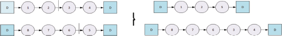
Figure 4. Operation mechanism of BCO algorithm
3.3. Adam-BCO
The Adam algorithm's inability to prevent local traps and the BCO's inability to examine different solution spaces, made the integration of both algorithms necessary. Integrating the Adam algorithm with the body change operator will further eliminate the weaknesses of both algorithms.
Actions are first produced as described in the Adam algorithm, to start the learning process with the proposed hybrid Adam-BCO algorithm. Algorithm 3 shows the mechanism of the proposed Adam-BCO algorithm.
Algorithm 3. Pseudocode of the Adam-BCO algorithm
Require: α: Step size, β1 and β2∈: decay rates for the moment estimates
Require:f(θ): Weight of deep-learning with parameters θ
Require: θ0: Initial weights of deep-learning and set to 0
m0 ← 0
ϑ0 ← 0
t ← 0 (Iteration (150))
while currentiteration < t do
t←t+1
If t%5 ← 0
perform: BCO algorithm to Gchp, Gchc
end if
while currentiteration < 50 do
perform: BCO algorithm to ch : {chp, chc}
end while
: Greedy rule
get the values of gradients (g(θt))
update first-moment estimate (mt)
update second-moment estimate (ϑt)
compute bias-corrected first moment estimâte (mt)
compute bias-corrected second moment estimâte (ϑt)
update weights (θt)
end while
returnend while θt
In the earlier chapters, randomly generated initial solutions create actions, and at the same time, actions refer to inputs. The parameters required by the Adam algorithm are specified, and the BCO algorithm improves the best solution in every five iterations. Thus, weight updates in the network are calculated according to the Adam algorithm. In addition to using the best solution in every five iterations, the BCO algorithm tries to improve the Greedy rule solutions obtained during the first 50 iterations. Regardless of whether the improvement is provided, the network weights are updated according to the mechanism of the Adam algorithm. Through the hybridization of both algorithms, it is ensured that more varied solution spaces are searched, and the Adam algorithm is not trapped in local solutions.
Figure 5 shows the Adam algorithm's operation mechanism for finding possible routings and scheduling. For the Adam-BCO hybrid algorithm to perform the learning action, feasible routing and scheduling are input as action. The best solution obtained in every five iterations is improved, and the weight is updated. Also, the solutions that are selected and created with the Greedy rule are improved in up to fifty iterations. Later, weights are updated, and the learning process that lasts 150 iterations is completed.
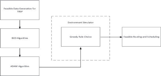
Figure 5. Operation mechanism of Adam-BCO algorithm in TRSP
4. Numerical Results
The Adam algorithm, the BCO method, and Adam-BCO hybrid algorithm are implemented in Python using a laptop with INTEL I5-3360M, a 2.80 GHz processor, and a 4 GB memory. A time windows technician dataset illustrates the performances of the three algorithms. The dataset includes 29 instances that consist of travel times, allowed days, time windows, proficiencies, 25 tasks, and one central depot. Table 2 illustrates the notation used in Table 3.
Table 2. The notation is used in Table 3
Instance |
Instance name |
Best Cost |
Best solution cost acquired by running algorithm ten times |
BKS |
Best known solution |
NBKS |
Number of best results acquired by the corresponding algorithm (bold) |
CPU Time |
A computational processing unit (Minute) |
Gap |
Percentage gap of the solution cost acquired by the related algorithm |
Ins |
Instance number |
Table 3. The instance results of the three algorithms
Dataset |
DL Algorithm |
Adam Algorithm |
BCO Algorithm |
Adam-BCO Algorithm |
||||||||||||||
Ins |
BKS |
Initial Solution |
Best Cost |
Usage of Depot |
Gap (%) |
CPU Time (min) |
Average Best Found |
Best Cost |
Usage of Depot |
Gap (%) |
CPU Time (min) |
Average Best Found |
Initial Solution |
Best Cost |
Usage of Depot |
Gap (%) |
CPU Time (min) |
Average Best Found |
C-101 |
230.10 |
297.18 |
259.70 |
5 |
12.86 |
0.06 |
273.69 |
258.70 |
5 |
12.43 |
1.71 |
275.45 |
303.25 |
231.20 |
5 |
0.44 |
5.38 |
247.06 |
C-102 |
227.60 |
284.96 |
259.80 |
5 |
14.15 |
0.06 |
272.80 |
233.10 |
5 |
2.42 |
2.52 |
251.26 |
292.48 |
234.60 |
5 |
3.08 |
5.65 |
245.01 |
C-103 |
227.60 |
288.83 |
243.40 |
5 |
6.94 |
0.06 |
275.74 |
233.30 |
5 |
2.50 |
4.84 |
246.63 |
276.19 |
227.60 |
5 |
0.00 |
5.80 |
242.17 |
C-104 |
225.70 |
260.05 |
229.80 |
5 |
1.81 |
0.06 |
256.34 |
229.90 |
5 |
1.86 |
8.23 |
243.10 |
266.32 |
225.70 |
5 |
0.00 |
5.63 |
233.68 |
C-105 |
230.10 |
291.90 |
281.60 |
6 |
22.38 |
0.07 |
287.90 |
239.20 |
5 |
3.95 |
18.75 |
251.95 |
282.86 |
239.20 |
5 |
3.95 |
6.14 |
248.46 |
C-106 |
230.10 |
302.48 |
257.30 |
5 |
11.82 |
0.08 |
293.75 |
248.60 |
5 |
8.04 |
2.02 |
271.99 |
307.49 |
230.10 |
5 |
0.00 |
6.49 |
255.04 |
C-107 |
278.80 |
333.73 |
296.90 |
5 |
6.49 |
0.09 |
316.53 |
292.70 |
5 |
4.99 |
2.02 |
316.82 |
346.03 |
280.50 |
5 |
0.61 |
4.38 |
332.16 |
C-108 |
278.80 |
350.94 |
301.30 |
6 |
8.07 |
0.07 |
339.62 |
280.50 |
5 |
0.61 |
0.31 |
336.51 |
330.77 |
280.00 |
5 |
0.43 |
1.67 |
318.66 |
C-109 |
277.30 |
344.17 |
316.90 |
6 |
14.28 |
0.09 |
331.11 |
317.30 |
6 |
14.42 |
0.25 |
337.58 |
330.24 |
284.90 |
5 |
2.74 |
0.56 |
312.46 |
R-101 |
440.20 |
518.67 |
442.40 |
5 |
0.40 |
0.09 |
458.67 |
447.60 |
5 |
1.68 |
3.16 |
458.60 |
495.80 |
445.80 |
5 |
1.27 |
7.37 |
459.49 |
R-102 |
421.00 |
525.38 |
457.30 |
5 |
8.62 |
0.09 |
500.30 |
436.80 |
5 |
3.75 |
12.88 |
464.22 |
495.82 |
435.70 |
5 |
3.49 |
7.63 |
452.60 |
R-103 |
406.30 |
490.43 |
418.40 |
5 |
2.98 |
0.07 |
457.78 |
424.30 |
5 |
4.43 |
2.90 |
433.97 |
482.81 |
412.70 |
5 |
1.58 |
6.47 |
432.62 |
R-104 |
404.30 |
490.31 |
439.60 |
5 |
8.73 |
0.08 |
459.46 |
416.20 |
5 |
2.94 |
9.28 |
426.24 |
494.56 |
406.30 |
5 |
0.50 |
6.64 |
436.01 |
R-105 |
490.80 |
620.66 |
516.90 |
6 |
5.32 |
0.10 |
559.81 |
520.70 |
6 |
6.09 |
3.14 |
556.05 |
604.15 |
511.20 |
6 |
4.16 |
5.39 |
542.15 |
R-106 |
476.40 |
584.63 |
498.90 |
5 |
4.72 |
0.10 |
534.63 |
487.00 |
5 |
2.23 |
4.93 |
537.00 |
636.48 |
480.30 |
5 |
0.82 |
6.63 |
530.28 |
R-107 |
476.40 |
594.49 |
508.60 |
5 |
6.76 |
0.11 |
562.09 |
513.80 |
5 |
7.85 |
2.01 |
528.06 |
590.67 |
499.30 |
5 |
4.81 |
6.42 |
550.67 |
R-108 |
470.60 |
592.45 |
501.60 |
5 |
6.59 |
0.10 |
557.24 |
514.40 |
5 |
9.31 |
2.24 |
550.87 |
598.11 |
498.30 |
5 |
5.89 |
6.74 |
555.62 |
R-109 |
480.60 |
595.73 |
546.60 |
5 |
13.73 |
0.12 |
565.15 |
552.00 |
5 |
14.86 |
1.70 |
566.05 |
592.55 |
543.40 |
5 |
13.07 |
2.86 |
567.95 |
R-110 |
480.60 |
600.72 |
552.70 |
5 |
15.00 |
0.09 |
579.41 |
551.70 |
5 |
14.79 |
0.54 |
557.40 |
611.11 |
556.40 |
5 |
15.77 |
0.24 |
569.96 |
R-111 |
478.30 |
620.88 |
494.20 |
5 |
3.32 |
0.11 |
542.88 |
500.80 |
5 |
4.70 |
6.83 |
519.25 |
595.49 |
515.40 |
5 |
7.76 |
7.53 |
525.90 |
R-112 |
395.30 |
486.35 |
417.40 |
5 |
5.59 |
0.10 |
436.14 |
413.80 |
5 |
4.68 |
0.55 |
435.49 |
479.65 |
395.30 |
5 |
0.00 |
6.15 |
421.69 |
RC-101 |
507.27 |
656.77 |
592.14 |
5 |
16.73 |
0.12 |
616.76 |
586.62 |
5 |
15.64 |
0.21 |
614.80 |
653.96 |
581.02 |
5 |
14.54 |
1.15 |
621.65 |
RC-102 |
475.14 |
662.99 |
552.28 |
6 |
16.24 |
0.23 |
592.69 |
586.89 |
6 |
26.83 |
0.22 |
607.84 |
667.68 |
572.99 |
6 |
20.59 |
0.26 |
601.08 |
RC-103 |
488.58 |
686.75 |
577.35 |
6 |
18.17 |
0.09 |
614.98 |
589.17 |
6 |
20.59 |
0.35 |
620.85 |
687.55 |
575.56 |
6 |
17.80 |
0.40 |
628.11 |
RC-104 |
482.42 |
732.71 |
546.92 |
5 |
13.37 |
0.13 |
586.51 |
560.66 |
5 |
16.22 |
0.33 |
594.65 |
681.12 |
561.44 |
5 |
16.38 |
0.17 |
589.70 |
RC-105 |
545.50 |
754.82 |
609.77 |
6 |
11.78 |
1.20 |
648.63 |
631.31 |
6 |
15.73 |
1.16 |
661.15 |
753.55 |
583.21 |
6 |
6.91 |
1.21 |
639.56 |
RC-106 |
510.33 |
720.23 |
599.04 |
6 |
17.38 |
0.09 |
610.72 |
571.47 |
6 |
11.18 |
0.25 |
599.53 |
741.71 |
559.43 |
6 |
9.62 |
0.63 |
604.15 |
RC-107 |
509.89 |
720.61 |
552.03 |
6 |
8.27 |
0.10 |
618.26 |
579.32 |
6 |
13.62 |
0.35 |
616.16 |
712.83 |
540.97 |
5 |
6.10 |
0.62 |
612.46 |
RC-108 |
553.35 |
692.88 |
594.18 |
6 |
7.38 |
0.23 |
620.25 |
595.11 |
6 |
7.55 |
1.15 |
614.51 |
694.75 |
575.03 |
6 |
3.92 |
0.72 |
609.51 |
Avg. |
403.43 |
520.78 |
443.62 |
5.35 |
9.99 |
0.14 |
474.82 |
441.83 |
5.28 |
8.82 |
3.27 |
465.31 |
517.45 |
430.47 |
5.21 |
5.73 |
4.03 |
461.58 |
NBKS |
|
|
0 |
|
|
|
|
0 |
|
|
|
|
|
3 |
|
|
|
|
Table 3 illustrates the comparison table of Adam, BCO, and Adam-BCO algorithms. The results in Table 3 show why the Adam method should be implemented with the BCO method. The starting and ending intervals of the daily working hours of the C, R, RC test sets are given as [0, 1236], [0, 230], [0, 240]. Working times, service times and time constraints of the three datasets differ. As a result of these differences, problem sets produce solutions at different solution values and times. The fact that the three primary datasets have different characteristics makes it possible to perform a better evaluation of the efficiency of the algorithms or hybrid methods to be applied.
Considering the average of the best solution values of the BCO algorithm and the Adam algorithm-based deep learning, it is seen that they are very close to each other. Adam algorithm-based deep learning produces feasible solutions with a 9.99% Gap and the BCO algorithm with an 8.82% Gap. It is crucial that the Adam algorithm-based deep learning obtain feasible solutions for TRSP with the specified Gap. Even methods that give exact and heuristic solutions do not guarantee optimal results and achieve higher solution times. Here, the average time for feasible solutions obtained with Adam algorithm-based deep learning is 0.14 minutes.
The aim is to integrate the Adam algorithm-based deep learning method with the BCO algorithm and obtain feasible solutions. With the randomness in the structure of the initial solutions required to reach different search spaces in the TRSP, the average initial solution values may differ, although not significantly. Some of the obtained initial solution values may be decent, and provide better solutions, nonetheless, in some cases, this does not give the possibility of searching for other solution spaces.
The Adam algorithm provides the average best cost of 443.62 units, and the average best found of 474.82 units. The BCO algorithm provides the average best cost of 441.83 units, and the average best found is 465.31 units. The Adam algorithm has been integrated with the BCO algorithm, and Adam-BCO based deep learning algorithm has been applied. Performing the hybrid algorithm provides the average best solution value as 430.47 units, and the average best found as 461.58 units. The average best value offers a difference of 5.71% Gap from the best solutions. The average solution time increases from 0.14 minutes to 4.03 minutes, but in return, Gap decreases from 9.99% to 5.71%. The performing hybridization of both algorithms based on deep learning provides effective feasible solutions considering the results.
5. Conclusions
This paper proposed an Adam-BCO hybrid algorithm to solve TRSP, which is a combinatorial optimization problem. The TRSP consists of assigning technicians to teams, assigning teams to tasks, creating routes, and the selected technician group that must meet certain level of qualification. The TRSP included a pre-determined set of technicians who have various talents and a set of tasks requested by the customer at various locations. To perform tasks consisting of customer requests, the set of technicians are divided into teams, and teams travelling in different locations are assigned to the tasks. The numerical results provide that the performance of the proposed Adam-BCO algorithm is experimentally compared with the separate performance of the Adam and BCO algorithms for the solution of the TRSP on Pekel's modified instances. The conclusions of this article are presented as follows:
• The Adam algorithm was caught on local traps, and the BCO method failed to examine different solution spaces. The two algorithms have been integrated to eliminate each other’s weaknesses, and the possibility of searching for new solution spaces has emerged. The changes are carried out to provide that the Adam algorithm-based deep learning method provides fast and ideal feasible solutions for TRSP.
• There are 26 hidden neurons in the first hidden layer. The main reason for choosing 26 neurons is that there are 25 customers and one central depot in the discussed TRSP. Since there are 26 nodes, 26 neuron and input entries are made. The number of hidden neurons would increase if the number of nodes addressed in the problem, the number of customers and depots increases.
• The Adam algorithm-based deep learning method can produce solutions close to optimal results in some data sets using the advantage of gradients' first and second moments, considering the parameters included in its structure.
• Although the Adam algorithm based deep learning method has a 9.99% Gap, it provides a swift solution using the advantage of the first and second moments of gradients, considering the parameters included in its structure.
• As a result of the randomness in the structure of the initial solutions required to solve the problem, the average initial solution values may differ, although not significantly. Some of the obtained initial solution values may be decent and provide better solutions, nonetheless, in some cases, this does not enable the search for other solution spaces.
• The deep learning method based on the Adam-BCO algorithm offers the best feasible solutions with a 5.73% Gap using the powerful sides of the two algorithms. While the Adam algorithm provides a faster approach to solution spaces, the BCO method explores those that could not be investigated before.
• The average best solution value obtained by the Adam-BCO algorithm-based deep learning method promises to reach better solutions in the future. With the combination of the strengths of both algorithms, more effective results have emerged. This situation shows the importance of integrating and researching other algorithms.
In future studies, better results can be obtained with the use of different learning algorithms in combinatorial problems such as TRSP. Also, a more effective solution space search can be performed by integrating heuristic methods and deep learning algorithms.
References
Anoshkina, Y., and Meisel, F. (2019). Technician Teaming and Routing with Service-, Cost-and Fairness-Objectives. Computers & Industrial Engineering.
Çakırgil, S., Yücel, E., and Kuyzu, G. (2020). An integrated solution approach for multi-objective, multi-skill workforce scheduling and routing problems, Computers & Operations Research 118: 104908.
Charris, E. L. S., Montoya-Torres, J. R., and Guerrero-Rueda, W. (2019). A decision support system for technician routing with time windows. Academia RevistaLatinoamericana de Administración.
Chen, X., Thomas, B. W., and Hewitt, M. (2016). The technician routing problem with experience-based service times. Omega, 61, 49–61.
Duchi, J., Hazan, E., and Singer, Y. (2011). Adaptive subgradient methods for online learning and stochastic optimization. The Journal of Machine Learning Research, 12:2121–2159.
Fu, T., Wang, C., and Cheng, N. (2020). Deep-learning-based joint optimization of renewable energy storage and routing in vehicular energy network. IEEE Internet of Things Journal, 7(7), 6229–6241.
Graf, B. (2020). Adaptive large variable neighborhood search for a multiperiod vehicle and technician routing problem. Networks, 76(2), 256–272.
Hernández-Jiménez, R., Cárdenas, C., and Rodríguez, D. M. (2019). Towards the Optimal Solution for the Routing Problem in Vehicular Delay Tolerant Networks: A Deep Learning Approach. IEEE Latin America Transactions, 17(12), 2028–2036.
Hussain, D., Khan, M. A., Abbas, S., Naqvi, R. A., Mushtaq, M. F., Rehman, A., and Nadeem, A. (2021). Enabling Smart Cities with Cognition Based Intelligent Route Decision in Vehicles Empowered with Deep Extreme Learning Machine. CMC-computers materials & continua, 66(1), 141–156.
James, J. Q., Yu, W., and Gu, J. (2019). Online vehicle routing with neural combinatorial optimization and deep reinforcement learning. IEEE Transactions on Intelligent Transportation Systems, 20(10), 3806–3817.
Khalfay, A., Crispin, A., and Crockett, K. (2017, September). A review of technician and task scheduling problems, datasets and solution approaches. 2017 Intelligent Systems Conference. pp. 288–296.
Kingma, D. P., and Ba, J. (2014). Adam: A method for stochastic optimization. arXiv preprint arXiv:1412.6980.
Koh, S., Zhou, B., Fang, H., Yang, P., Yang, Z., Yang, Q., and Ji, Z. (2020). Real-time deep reinforcement learning based vehicle navigation. Applied Soft Computing, 96, 106694.
Kovacs, A., Parragh, S. N., Doerner, K. F., and Hartl, R. F. (2012). Adaptive large neighborhood search for service technician routing and scheduling problems. Journal of scheduling, 15(5), 579–600.
Lee, K. B., A Ahmed, M., Kang, D. K., and Kim, Y. C. (2020). Deep Reinforcement Learning Based Optimal Route and Charging Station Selection. Energies, 13(23), 6255.
Mathlouthi, I., Gendreau, M., and Potvin, J. Y. (2021). A metaheuristic based on Tabu search for solving a technician routing and scheduling problem. Computers & Operations Research, 125, 105079.
Mathlouthi, I., Gendreau, M., and Potvin, J. Y. (2018). Mixed integer linear programming for a multi-attribute technician routing and scheduling problem. INFOR: Information Systems and Operational Research, 56(1), 33–49.
Pekel, E. (2020). Solving technician routing and scheduling problem using improved particle swarm optimization. Soft Computing, 24(24), 19007–19015.
Pekel, E., and Kara, S. S. (2019). Solving fuzzy capacitated location routing problem using hybrid variable neighborhood search and evolutionary local search. Applied Soft Computing, 83, 105665.
Tieleman, T. and Hinton, G. (2012). Lecture 6.5 - RMSProp, Coursera: Neural Networks for Machine Learning. Technical report.
Wang, J., and Sun, L. (2020). Dynamic holding control to avoid bus bunching: A multi-agent deep reinforcement learning framework. Transportation Research Part C: Emerging Technologies, 116, 102661.
Whitley, D. (1994). A genetic algorithm tutorial. Statistics and computing, 4(2), 65–85.
Zamorano, E., and Stolletz, R. (2017). Branch-and-price approaches for the multiperiod technician routing and scheduling problem. European Journal of Operational Research, 257(1), 55–68.