
Regular Issue, Vol. 10 N. 3 (2021), 307-320
eISSN: 2255-2863
DOI: https://doi.org/10.14201/ADCAIJ2021103307320
|
ADCAIJ: Advances in Distributed Computing and Artificial Intelligence Journal
Regular Issue, Vol. 10 N. 3 (2021), 307-320 eISSN: 2255-2863 DOI: https://doi.org/10.14201/ADCAIJ2021103307320 |
Deep Convolutional Neural Network Modeling and Laplace Transformation Algorithm for the Analysis of Surface Quality of Friction Stir Welded Joints
Akshansh Mishraa, Anusri Pattib
a Centre for Artificial Intelligent Manufacturing Systems, Stir Research Technologies, India
b Department of Computer Sciences and Engineering, SRM Institute of Science and Technology, Kattangulathur, India
akshansh.frictionwelding@gmail.com, pl.anusree.2000@gmail.com
ABSTRACT
The quality of Friction Stir Welded joint depends on the input parameters like tool rotational speed, tool traverse speed (mm/min), tool tilt angle and an axial plunge force. If there is any variation in these input parameters then there will be a chance of formation of various surface defects such as groovy edges, flash formation and non-homogenous mixing of alloys. The main objective of the present work is use machine learning algorithms such as Deep Convolutional Neural Network (DCNN) and Laplace transformation algorithm to detect these surface defects present on the Friction Stir Welded joint. The results showed that the used algorithms can easily detect such surface defects with good accuracy.
KEYWORDS
Machine Learning, Friction Stir Welding, Convolutional Neural Network, Surface Defects, Laplace Algorithm
1. Introduction
A digital image as shown in Figure 1 is a two-dimensional function i.e. f(x,y) where x and y are plane coordinates which are height and width and f is the amplitude at any pair of coordinates (x,y) i.e. the brightness of the given image.
A digital image is a collection of a finite number of pixels in different color spaces which is the smallest element of an image that has a particular location and value. If any digital image is zoomed to such an extent that small squares are visible then those small squares observed are pixels as shown in Figure 2.
It should be noted that each pixel in a given image has a different position and value which can be the color range that is between (0,255). The mechanism of digital image formation is shown in Figure 3. Firstly, a device i.e. camera is required to capture the image of a given object in presence of a particular source of energy that emits light. Secondly, a sensor is needed for image acquisition purposes i.e. for capturing the structure of a given object. When a given structure of an object is under acquisition by a sensor then it will generate a continuous voltage signal which is generated by the amount of sensed data. Sampling and Quantization are subjected to the generated continuous voltage signal. Sampling is the process of digitizing the coordinate value i.e. number of pixels per unit area. Quantization refers to digitizing the amplitude value of the generated continuous voltage signal i.e. the analog to the digital conversion of an input image f(x,y).
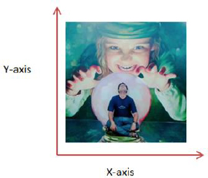
Figure 1: Representation of a digital image in two-dimensional form
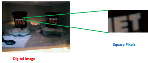
Figure 2: Representation of the pixels in a given digital image after zooming in

Figure 3: Mechanism of Digital Image generation
2. Working Mechanism of Deep Convolutional Neural Network
It should be noted that the pixels are arranged in a form of matrix known as RGB image that contains three layers of two-dimensional image, these layers are Red, Green, and Blue channels as shown in Figure 4.

Figure 4: Schematic representation of RGB Channels
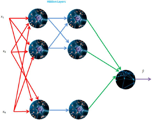
Figure 5: Neural Network architecture
One of the challenges in computer vision is that number of inputs can get really big. Suppose we have an image of dimensions 64 X 64 X 3, after multiplication we are going to get the input feature dimensions as 12288. But then things get complicated when we work with larger images such 1000 as pixels X 1000 pixels X 3 RGB channels after multiplication we are going to get the input dimension as 3 million. So if we have 3 million input features then x, as shown in Figure 5, will be 3 million dimensional and the first hidden layer may have approximately 1000 hidden units then the total number of weights i.e. the matrix w[1] if we use standard fully connected network then this matrix will be (1000, 3 million) dimensional matrix because x∈R3million which means that the obtained matrix will have 3 billion parameters which are very very large. So these obtained large number of parameters is difficult to obtain enough data to prevent a Neural Network from overfitting and also the requirement of computational and memory power to process these humongous parameters is infeasible.
Padding is one of the modifications to the basic convolutional operation in order to construct the Deep Neural Network. It is normally observed that if we take a 5 X 5 image (n X n format) and convolve it with a 2 X 2 (f X f format) filter then we will get a 4 X 4 (n-f+1 X n-f+1 format) matrix as an output because the number of possible positions for the 2 X 2 filter there are only 4 X 4 possible positions for 2 X 2 filter to fit in 5 X 5 image matrix as shown in Figure 6. It should be noted that whenever the convolutional operator i.e. ‘*’ is applied then there is a shrinkage in the image and another disadvantage is that there is major information lost at the edge of the images. So in order to solve the shrinkage output and loss of information from the problem of the edges, we can pad the image by the addition of one pixel around the image as shown in Figure 7.
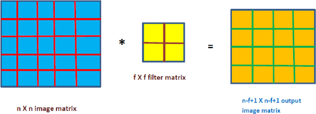
Figure 6: Convolution of filter over input image
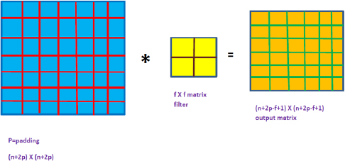
Figure 7: Convolution of filter over padded input image
The amount of padding is decided by two factors i.e. valid convolutions and same convolutions. There is no need for padding in the case of valid convolutions which is governed by the following equation:
In the case of the same convolutions, the size of output size is the same as the input size. So the following calculation is made to find out the amount of padding required:
where ‘p’ is the amount of padding required in equation 3 and ‘f’ is usually an odd valued filter.
Figure 8 shows the mechanism of the construction of one layer of a convolutional neural network. It is observed that when a three-dimensional input image is convolved with two different three-dimensional filters it results in two different output images. In order to include the resulted image in a convolutional layer, bias is added which can be any real number, and then a non-linearity is applied such as ReLu and it results in an output image, and the resulted final images are stacked up to form one layer of a convolutional neural network.
In this analogy the input image is represented as a[0] and the applied filters are considered as w[1]. So when the mapping operation is done between the filters and the input image then it can be represented as equation 4.
When non-linearity activation function is introduced then it can be represented by equation 5. Equation 5 becomes the activation for a next layer.
If layer l is a convolutional layer then the filter size is denoted by f[l], the amount of padding is denoted by p[l] and the stride is denoted by s[l]. The input to this convolutional layer is going to be in dimensions denoted by while the output image yielded by this convolutional layer will be of dimension . For calculating and , Equation 6 and 7 are used.
3. Related Work
Nowadays, Machine Learning has one of the fastest-growing applications in the manufacturing and materials industries. Machine Learning techniques are being implemented for engineering design, development, and also for determining the mechanical and microstructure properties of the fabricated mechanical components. Yosipof et al. [1] constructed the machine learning-driven approach for the production of solar cell libraries based on Titanium and Copper oxides. Tawfik et al. [2] used a machine learning approach for the prediction of quantum mechanical thermal properties of crystals. Machine learning algorithms have a wide application for predicting mechanical properties such as Ultimate Tensile Strength, Elongation, and Fracture strength [3–8].
Likely other manufacturing operations, the Friction Stir Welding process is also being subjected to various types of machine learning algorithms. The process of machine learning greatly reduces the time it takes to develop powerful, simple materials. This is important in the aerospace, automotive and manufacturing sectors. Mechanical learning techniques such as Artificial Neural Networks and Image processing are used in the Friction Stir Welding process for the optimization of structures such as Ultimate Tensile Strength, Fracture Strength and elongation% and microstructure structures such as grain size and understanding of error formation [9-12].
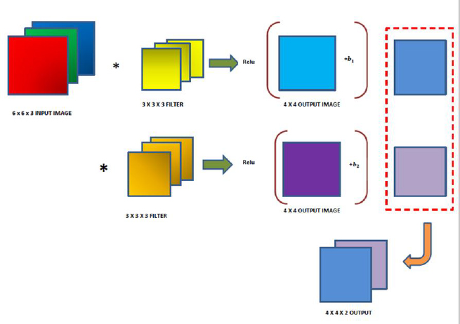
Figure 8: Construction of a single Convolutional Layer
Verma et al. [13] used a variety of sophisticated machine learning methods such as. Gaussian regression (GP) regression process, support vector machining (SVM), and multi-linear regression (MLR) to test the process of welding the pressure force. It was observed that the GPR method works better than the SVM and MLR methods. Therefore, the GPR method is used effectively to predict UTS welding of welded joints.
Friction Stir Welded joint is not free from various surface defects such as micro-crack formation, groovy edges, voids, pores, and flash formation due to improper selection of input parameters such as tool rotational speed (rpm), tool traverse speed (mm/min) and tool tilt angle, etc. There is a limited literature survey available on the application of CNN model in Friction Stir Welding Process. The present work focuses on the development of a Deep Convolutional Neural Network and Laplace algorithm to trace such defects present in Friction Stir Welded joints.
4. Material and Methods
The dataset was collected in a folder having two sub-folders titled "good quality joint" and "bad quality joint". The dataset consisted of images having defects as well as images with no defects. As the data was very limited, Image Augmentation has been used to expand the dataset. The augmented images of bad surface joint and good surface joint are shown in Figure 9 and 10.
The path of the folder or drive was set that has all the images stored, and listed the names of the images stored. Next the ImageDataGenerator function was defined with the parameters as the operations to be performed. A function with the arguments is further defined as path to images and path to store the newly generated images. It calls the new_img function and stores the newly generated images in the given directory and also prints the number of images printed. The variables were declared which hold the path to the newly generated images, and call the create_new_images functions. The dataset is prepared in which 1000 images are used for training purpose and 400 images are used for testing purpose. These operations are performed in Google Colaboratory environment by using Python Coding.
The cropped image is further uploaded to the Google Colaboratory platform and it is subjected to machine learning-based image techniques i.e. Laplacian Operator. Figure 11 shows the step by step procedure to which the cropped image is being subjected during Laplace transformation.
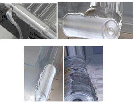
Figure 9: Sample of augmented images of bad surface quality

Figure 10: Augmented image of Good quality joint

Figure 11: Laplace Operator subjected to cropped image of Friction Stir Welded Joint
5. Results and Discussion
5.1. Deep Convolutional Neural Network
Figure 12 shows the Deep Convolutional Neural Network (DCNN) structure used in the recent research. The dimension of the images i.e. width and height has been set to 150 pixels. An explicit assumption is made by the DCNN architecture by assuming the inputs in form of images which inculcates the encoding process in the given architecture.
The first convolutional layer is applied to get 32 feature maps by using 3 by 3 kernel where the input image is 150px by 150 px and has 3 channels for the coloured image. The activation function used is reLu which helps with non-linearity in the neural network. Next, there is addition of another layer max pooling which reduces the number of cells and helps detect features like colors, edges etc. The pool size of 2 by 2 is used for all 32 feature maps. Next, the data is flattened and it is sent as input to the network. A fully connected neural network was built with 64 input units and one output unit with a dropout rate of 0.5, and as this is a binary classification problem we use the sigmoid activation function in the output layer. Now, the neural network is compiled with loss function “binary_crossentropy” as it is a binary classification problem and we use the “rmsprop” optimizer which increases the learning rate of our algorithm and accelerates the convergence. Random transformations are applied on the images using image augmentation and create the final train and test set. Figure 13 shows the plot between the accuracy of training and validation data. It is observed that the accuracy of training data is 0.98 and validation data is 0.95. Figure 14 shows the variation of loss function with increasing number of epochs.
Limitation of the DCNN architecture is that it requires large training dataset for resulting good accuracy score and also maxpool operation involved in DCNN mechanism makes the architecture slow.
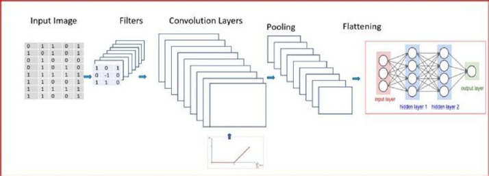
Figure 12: Deep Convolutional Neural Network Architecture
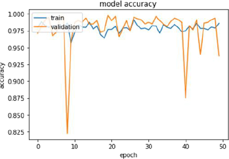
Figure 13: Plot of training and validation set accuracy

Figure 14: Plot of loss function with respect to number of epochs
5.2. Laplace Operator Algorithm
Equation 8 defines the Laplacian operator.
Where the partial first order derivative in the x-direction is as follows:
And in y-direction is given as follows:
After combining Equation 9 and Equation 10, we obtain a second derivative operator i.e. Laplacian Operator as shown in Equation 11.
Laplace filter can easily be constructed based on Equation 11 as shown below.
F(x-1,y-1) |
F(x-1,y) |
F(x-1,y+1) |
F(x,y-1) |
F(x,y) |
F(x, y+1) |
F(x+1,y-1) |
F(x+1,y) |
F(x+1,y+1) |
In the recent work, we have used Laplace 4-neighborhood and 8-neighborhood operator as shown below.
The image obtained is shown in Figure 15. It is observed that Laplace 8-neighborhood filter provides better quality image resolution and the characteristics such as surface defects present on Friction Stir Welded joint can be better inferred in comparison to Laplace 4-neighborhood filter operator.
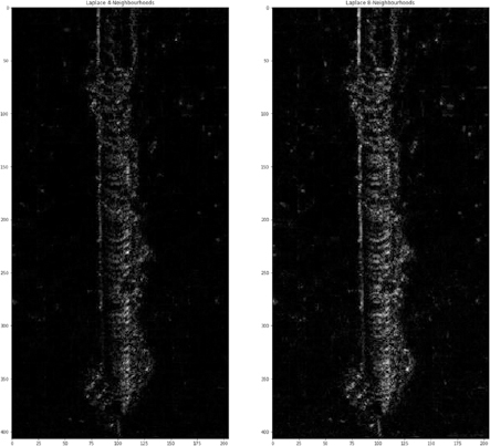
Figure 15: Cropped image undergone Laplace transformation
6. Conclusion
The recent work has implemented the concept of Deep Convolutional Neural Network algorithm and also a machine learning based image processing techniques Laplace transform operator. The results showed that the surface defects present on the Friction Stir Welded joint can be successfully detected by using Deep Convolutional Neural Network model with an accuracy of 95 percent. It is also observed that Laplace 8-neighborhood transform yields better result than Laplace 4-neighborhood operator. There were limited dataset for obtaining more accuracy score. The future work which can be worked upon this algorithm is the real time monitoring and inspection of the surface defects in welded joints.
7. References
[1] Yosipof, A., Nahum, O.E., Anderson, A.Y., Barad, H.N., Zaban, A. and Senderowitz, H., 2015. Data Mining and Machine Learning Tools for Combinatorial Material Science of All-Oxide Photovoltaic Cells. Molecular informatics, 34(6-7), pp.367-379.
[2] Tawfik, S.A., Isayev, O., Spencer, M.J. and Winkler, D.A., 2020. Predicting thermal properties of crystals using machine learning. Advanced Theory and Simulations, 3(2), p.1900208.
[3] Jiang, X., Jia, B., Zhang, G., Zhang, C., Wang, X., Zhang, R., Yin, H., Qu, X., Song, Y., Su, L. and Mi, Z., 2020. A strategy combining machine learning and multiscale calculation to predict tensile strength for pearlitic steel wires with industrial data. Scripta Materialia, 186, pp.272-277.
[4] Behnood, A. and Golafshani, E.M., 2020. Machine learning study of the mechanical properties of concretes containing waste foundry sand. Construction and Building Materials, 243, p.118152.
[5] Bai, B., Han, X., Zheng, Q., Jia, L., Zhang, C. and Yang, W., 2020. Composition optimization of high strength and ductility ODS alloy based on machine learning. Fusion Engineering and Design, 161, p.111939.
[6] Xie, Q., Suvarna, M., Li, J., Zhu, X., Cai, J. and Wang, X., 2020. Online prediction of mechanical properties of hot rolled steel plate using machine learning. Materials & Design, p.109201.
[7] Xu, X., Wang, L., Zhu, G. and Zeng, X., 2020. Predicting Tensile Properties of AZ31 Magnesium Alloys by Machine Learning. JOM, pp.1-8.
[8] Zhang, J., Sun, Y., Li, G., Wang, Y., Sun, J. and Li, J., 2020. Machine-learning-assisted shear strength prediction of reinforced concrete beams with and without stirrups. Engineering with Computers, pp.1-15.
[9] Mishra, A. (2020). Local binary pattern for the evaluation of surface quality of dissimilar Friction Stir Welded Ultrafine Grained 1050 and 6061-T6 Aluminium Alloys. ADCAIJ: Advances in Distributed Computing and Artificial Intelligence Journal, 9(2), 69-77. https://doi.org/10.14201/ADCAIJ2020926977
[10] Mishra, A., & Pathak, T. (2020). Estimation of Grain Size Distribution of Friction Stir Welded Joint by using Machine Learning Approach. ADCAIJ: Advances in Distributed Computing and Artificial Intelligence Journal, 10(1), 99-110. https://doi.org/10.14201/ADCAIJ202110199110
[11] Mishra, A. 2020. “Artificial Intelligence Algorithms for the Analysis of Mechanical Property of Friction Stir Welded Joints by using Python Programming”, Weld. Tech. Rev., vol. 92, no. 6, pp. 7-16, Aug. 2020.
[12] Mishra, A., 2020. Discrete Wavelet Transformation Approach for Surface Defects Detection in Friction Stir Welded Joints. Fatigue of Aircraft Structures, 1(ahead-of-print).
[13] Verma, S., Misra, J.P., Singh, J., Batra, U. and Kumar, Y., 2021. Prediction of tensile behavior of FS welded AA7039 using machine learning. Materials Today Communications, 26, p.101933.
GitHub Repository Link
https://github.com/akshansh11/CNN-Model-for-Bad-quality-FSW-surface-analysis