
Regular Issue, Vol. 10 N. 4 (2021), 419-434
eISSN: 2255-2863
DOI: https://doi.org/10.14201/ADCAIJ2021104419434
|
ADCAIJ: Advances in Distributed Computing and Artificial Intelligence Journal
Regular Issue, Vol. 10 N. 4 (2021), 419-434 eISSN: 2255-2863 DOI: https://doi.org/10.14201/ADCAIJ2021104419434 |
Ensemble Boosted Tree based Mammogram image classification using Texture features and extracted smart features of Deep Neural Network
Bhanu Prakash Sharmaa and Ravindra Kumar Purwara
a Guru Gobind Singh Indraprastha University, New Delhi-India
bhanu.12016492317@ipu.ac.in, ravindra@ipu.ac.in
ABSTRACT
Inspired from the fact of breast cancer statistics that early detection reduces mortality and complications of later stages; in this paper, the authors proposed a technique of Computer-Aided Detection (CAD) of breast cancer from mammogram images. It is a multistage process which classifies the mammogram images into benign or malignant category. During preprocessing, images of Mammographic Image Analysis Society (MIAS) database are passed through a couple of filters for noise removal, thresholding and cropping techniques to extract the region of interest, followed by augmentation process on database to enhance its size. Features from Deep Convolution Neural Network (DCNN) are merged with texture features to form final feature vector. Using transfer learning, deep features are extracted from a modified DCNN, whose training is performed on 69% of randomly selected images of database from both categories. Features of Grey Level Co-Occurrence Matrix (GLCM) and Local Binary Pattern (LBP) are merged to form texture features. Mean and variance of four parameters (contrast, correlation, homogeneity and entropy) of GLCM are computed in four angular directions, at ten distances. Ensemble Boosted Tree classifier using five-fold cross-validation mode, achieved an accuracy, sensitivity, specificity of 98.8%, 100% and 92.55% respectively on this feature vector.
KEYWORDS
Mammogram; Transfer Learning; Deep Convolution Neural Network; Texture feature; LBP; GLCM
1. Introduction
According to a report published by (Sung et al., 2020) in GLOBOCAN for 2020, there are 19.3 million cases of cancer and out of it 10 million deaths are recorded. For breast cancer, this count is 2.3 million of total. Earlier, in order to control breast cancer, Randomized Controlled Trials (RCT's) were done, in which screening was done randomly, which reduced the mortality rate of breast cancer, but the rate of its incidents was unchanged. So, many countries suggested mammogram scanning regularly (once in 2-3 years). A report published by (Dibden et al., 2020) states that attending such screening reduced the death rate by 30%. Indian Council of Medical Research (ICMR) published India's cancer statistics in (Mathur et al., 2020; Song et al., 2020), according to which 1392179 was the total number of cancer patients for the year 2020. Further, breast cancer was among the top 5 leading categories of cancer, and 1 in 29 females supposed to develop breast cancer.
A mammogram image is generated by passing X-ray light through the breast of the patient. A mammogram represents the breast's internal view, from which it becomes possible to detect the presence of lumps/ tumors. Earlier, mammograms were checked manually by radiologists, but recently several Computer-Aided Detection (CAD) techniques are being developed to automate this process. Based on a mammogram image, these techniques classify the corresponding breast either in cancerous (malignant) or non-cancerous (benign) category.
Research using various techniques has already been done and still going on to improve this CAD process further. In (Sannasi & Rajaguru, 2020), authors suggested extraction of eight statistical features including mean, median and mode from preprocessed mammograms of the MIAS database. Firefly algorithm (FA), Extreme learning machine (ELM), Least Square based nonlinear regression (LSNLR) models achieved accuracies of 86.75%, 90.83%, and around 93%, respectively. To reduce misclassification cases, authors in (Boudraa et al., 2020) suggested a super-resolution reconstruction technique to reinforce the multi-stage CAD system's statistical texture features. It achieved a classification accuracy of 96.7%. Authors in (Mohanty et al., 2020) shared a multi-stage CAD technique. A block-based Cross Diagonal Texture Matrix (CDTM) is applied to the mammogram's Region of Interest (ROI), followed by extraction of Haralick's feature. Feature vector's dimension reduced using kernel principal component analysis (KPCA). They proposed a wrapper-based kernel extreme learning machine (KELM) technique; Grasshopper Optimization used to compute its parameter's optimized value. It achieved the classification accuracy of 97.49% for MIAS and 92.61 for the DDSM database, respectively.
Significant work has been proposed in literature over existing approaches using various Machine Learning (ML) techniques like Deep Learning (DL), Transfer Learning (TL), Convolution Neural Network (CNN), Deep CNN (DCNN), and others. In (Song et al., 2020) authors used a DCNN model to extract score features. These features are merged with GLCM and Histogram of Oriented Gradient (HOG) features to form the final Feature Vector (FV). An accuracy of 92.80% has been claimed using decision tree based extreme gradient boosting (XGBoost) classification. In (Sharma et al., 2020), authors suggested an approach to find the ROI using dual thresholding techniques applied parallelly on preprocessed mammograms. One thresholding is done using Otsu's approach, while another is based on maximizing the inter class standard deviation. Using modified Alexnet DCNN, accuracy of 93.45% is obtained. In another approach, authors in (Sha et al., 2020) used the CNN-based Grasshopper Optimization Algorithm (GOA). GOA is a new stochastic swarm-based optimization algorithm; it starts with a random swarm of the population (local solutions) to find the global optimum solution. An accuracy of 92% achieved using this approach. In (Azlan et al., 2020), authors used wavelet filters for image denoising, which is followed by image enhancement using the top and bottom hat technique. Snake boundary detectors are used for segmentation, followed by augmentation to enhance the dataset. Features are extracted using DCNN, and Principal Component Analysis (PCA) is used for dimension reduction. Using 10-fold Cross-validation on Support Vector Machine (SVM), it achieved an overall accuracy of 95.24%.
Table 1 summarizes various breast cancer detection method along with their claimed accuracy for classification. A number of classifiers have been used and the maximum accuracy that has been claimed is closed to 97%, which shows that there is still a scope of improving accuracy for breast cancer detection in mammogram images. There are few techniques in literature which have evaluated the performance of the model by amalgamating external features as well as CNN extracted features.
Table 1: Summary of various breast cancer detection methods in mammograms
Techniques |
Brief description |
Accuracy |
Eight statistical features using mean, median, mode etc are used and performance of FA, ELM, LSNLR models has been studied. |
3.75%- FA 90.83%- ELM 93%- LSNLR |
|
A super resolution reconstruction technique to reinform the multi-stage CAD system’s statistical texture features. |
96.7% |
|
Cross diagonal texture matrix (CDTM) of mammogram ROI is used for extracting Haralick’s feature. |
97.49% |
|
A DCNN model is used to extract score features which are merged with GLCM and HOG features and performance of decision tree based XG-Boost classifier is evaluated. |
92.8% |
|
A dual thresholding method is used- one is based on otsu thresholding and another based on maximizing inter-class standard deviation. Alexnet DCNN is used for classification. |
93.45% |
|
Features extracted from DCNN are taken and PCA is used for dimensionality reduction. A 10-fold cross validation on SVM is used. |
95.24% |
Emerging technologies have significant growth in controlling breast cancer mortality, but improvement is still required. Improvement in the treatment of breast cancer is only possible if detected at an early stage. It has been observed through literature survey that it is not only necessary to detect breast cancer in early stages but also it should be detected accurately. In this direction, a method of early and more accurate detection of breast cancer in mammogram images has been proposed. In this method some external features like contrast, homogeneity, entropy and correlation of mammogram image are merged along with smart features extracted from a modified Deep CNN. Section 2 of this paper, describes the proposed method which is followed by experimental results in section 3. Section 4 covers the conclusion and future scope.
2. Proposed Work
The proposed approach of cancer detection in mammogram images is a multistage process which is summarized in figure 1 and explained below.
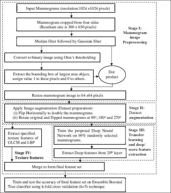
Figure 1: Block diagram of proposed work
2.1. Mammogram Preprocessing (Stage I)
Input: Raw mammogram images.
Output: preprocessed mammogram images.
When mammogram images are captured, the possibility of noise inclusion due to environmental, technical, and external factors is there. Among noises, two are very common; one is Gaussian noise due to the illumination and temperature of electronic parts, whereas another is present as salt and pepper noise. In this work, median and gaussian filters are used over others as their combination removes both of these noises while preserving maximum image information. In addition to this, to distinguish the mammograms, detail of the patient like id, name, date of capturing, view of the mammogram, the radiologists add markers and labels to the captured mammograms. Such labeling may be helpful if a mammogram image is inspected manually, but for automated systems, such unwanted information and noise adversely impact the classification accuracy. So, it is essential to focus only on the mammogram's suspicious region, i.e., ROI, and discard the remaining. In this work, to prepare the input greyscale images (1024x1024 pixels) for further process of feature extraction, they are passed through a couple of filters followed by process of ROI extraction and resizing to form enhanced images of 64x64 pixels as shown in figure 2 followed by its description:
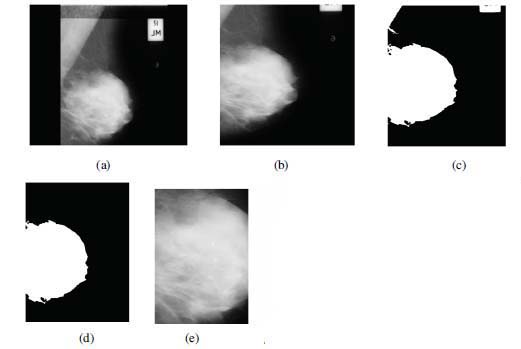
Figure 2: (a) Originally captured mammogram image along with identification labels. (b) Mammogram within bounding box of (300,200) and (600,850) is cropped followed by Median and Gaussian filtering. (c) Binary conversion of mammogram. (d) Identification of largest object from binarized mammogram. (e) ROI identified from mammogram in ‘b’ using the bounding box identified from mammogram in ‘d’.
1. When a mammogram is captured, markers and labels are added to it, as shown in figure 2(a).
2. On sides of mammogram, some region is non-usable (presence of straight lines, markers, black/ empty area). To reduce non-usable area, cropping of mammograms (1024x1024 pixels) from all four sides is performed and cropped image of size 300x650 pixels is obtained. Afterwards, the cropped mammogram image is processed using median filter (Ko & Lee 1998) and gaussian filter (Young & van Vliet 1995) to remove the salt and pepper noise and smoothen the edges. Figure 2(b) shows the result of step 2.
3. Binarize the mammogram using Otsu's thresholding technique (Otsu et al., 1979) as shown in figure 2(c).
4. Identify largest object from this binarized mammogram, keep it and discard other objects as shown in figure 2(d). Compute the bounding box of this object.
5. Based on the coordinates of this bounding box, retain the corresponding region (ROI) from the grey-scale image (step 2) and discard the remaining area.
6. To meet the input dimensions of the designed network, resize the retained ROI to 64x64 pixels. It is represented in figure 2(e). This resultant image is further used for image augmentation process.
2.2. Dataset Augmentation (Stage II)
Input: Preprocessed mammogram images.
Output: Augmented mammograms images.
The Mammographic Image Analysis Society (MIAS) dataset from (Suckling et al., 1994) is used for augmentation and evaluation purpose. In MIAS, mammograms are divided into normal, benign (most probably non-cancerous), and malign (most probably cancerous). In this work, normal and benign mammograms are clubbed into a single category as benign only, whereas remaining are considered as malignant. MIAS consists of a total of 322 mammograms, of which 270 are benign and 52 malign. These mammograms are of resolution 1024x1024 pixels. After preprocessing operations of step 2.1, resultant images of mammogram's ROI are of 64x64 pixels resolution. To increase the effectiveness of training and testing of proposed work, a large dataset is required. Hence image augmentation technique discussed in (Omonigho et al., 2020; Khan et al., 2019; Zhang et al., 2018) is used. Image augmentation is the process of using transformation techniques (like scaling, rotation, flip etc.) to create multiple transformed copies of the input image, thus increasing the number of cases forming the dataset. In the augmentation process (flip and rotation) used in this work, 322 input mammograms of resolution 64x64 are flipped horizontally, thus doubling the count from 322 to 644. Further, these 644 mammograms rotated at an angle of 90, 180 and 270 degrees to generate three different copies of each mammogram. So, 644 mammograms and their additional transformed copies make a total of 2576 resultant mammograms in the prepared/ augmented dataset. This augmented dataset covers the mammograms from different views and improves network learning and feature extraction.
2.3. Transfer learning and deep feature extraction (Stage III)
Input: Augmented mammogram images.
Output: Score/ deep DCNN features.
Once the dataset is ready, the next goal is to extract good quality features from it. From the modified DCNN shown in table 2, different values for layer activation and learnable parameters are used in hidden layers to extract deep features. It is helpful in extraction of quality feature from augmented/ prepared dataset over texture features extracted alone. Thus, in the proposed work, to enhance FV quality, GLCM and LBP's texture features are merged with deep features (DF) to form the final FV. In (Zhang et al., 2018), the authors suggested a transfer learning approach in which one model uses the information provided by the other. Inspired from it, DF extracted using transfer Learning technique on modified DCNN model. The detailed process of feature extraction is summarized below:
Table 2: Layers of modified Deep Neural Network
S. No. |
Layer Name |
Layer Description |
Layer Activation |
Learnable Parameters |
1 |
Image Input |
64x64x1 images with zero center normalization |
64x64x1 |
- |
2 |
Convolution |
96, 5x5 filter with stride [2 2] and padding [0 0 0 0] |
30x30x96 |
Weight: 5x5x1x96 Bias: 1x1x96 |
3 |
ReLU |
Rectifier Linear Unit |
30x30x96 |
- |
4 |
Cross Channel Normalization |
Cross channel normalization with 5 channels per element. |
30x30x96 |
- |
5 |
Max Pooling |
3x3 max pooling with stride [2 2] and padding [0 0 0 0]. |
14x14x96 |
- |
6 |
Convolution |
256, 5x5 filter with stride [1 1] and padding [2 2 2 2] |
14x14x256 |
Weight: 5x5x96x256 Bias: 1x1x256 |
7 |
ReLU |
Rectifier Linear Unit |
14x14x256 |
- |
8 |
Cross Channel Normalization |
Cross channel normalization with 5 channels per element. |
14x14x256 |
- |
9 |
Max Pooling |
3x3 max pooling with stride [2 2] and padding [0 0 0 0]. |
6x6x256 |
- |
10 |
Convolution |
384, 3x3 filter with stride [1 1] and padding [1 1 1 1] |
6x6x384 |
Weight: 3x3x256x384 Bias: 1x1x384 |
11 |
ReLU |
Rectifier Linear Unit |
6x6x384 |
- |
12 |
Convolution |
384, 3x3 filter with stride [1 1] and padding [1 1 1 1] |
6x6x384 |
Weight: 3x3x384x384 Bias: 1x1x384 |
13 |
ReLU |
Rectifier Linear Unit |
6x6x384 |
- |
14 |
Convolution |
256, 3x3 filter with stride [1 1] and padding [1 1 1 1] |
6x6x256 |
Weight: 3x3x384x256 Bias: 1x1x256 |
15 |
ReLU |
Rectifier Linear Unit |
6x6x256 |
- |
16 |
Max Pooling |
3x3 max pooling with stride [2 2] and padding [0 0 0 0]. |
2x2x256 |
- |
17 |
Fully Connected (FC1) |
4096 Fully connected layer. |
1x1x4096 |
Weight: 4096x1024 Bias: 4096x1 |
18 |
ReLU |
Rectifier Linear Unit |
1x1x4096 |
- |
19 |
Dropout |
50% Dropout. |
1x1x4096 |
- |
20 |
Fully Connected (FC2) |
4096 Fully connected layer. |
1x1x4096 |
Weight: 4096x4096 Bias: 4096x1 |
21 |
Softmax |
Softmax. |
1x1x4096 |
- |
22 |
Classification Output |
Classifies the input into one of two given classes using Cross entropy. |
- |
- |
Deep feature extraction using transfer learning:
In this work, deep features refer to those features that are extracted from the DCNN model. In (Omonigho et al., 2020), authors proposed a modified version of the Alexnet model, which has been taken as a reference model in this work. This DCNN architecture has been modified and deep features extracted from FC2 layer (shown at Serial no. 20 in table 2) are considered. In the referenced model, three layers (ReLU, Dropout, FC3) followed by FC2 are not contributing enough in terms of feature extraction and their removal reduces the network training time, therefore these layers have been dropped in the modified DCNN. The architecture of the modified DCNN is summarized in table 2.
In table 2, S.No. represents the sequence/ order of the layer's connections. Layer name represents the name and type of layers. Learnable parameters are the parameters that DCNN learns during training. Due to the optimization of these parameters during the training process, they are also known as trainable parameters. In modified DCNN model, Stochastic Gradient Descent (SGD) method is used for learning and optimization of learnable parameters (weights and biases of fully connected and convolution layers). Layer activations represent the outputs of layers.
This model accepts single channel (greyscale) images of size 64x64. Different Convolution layers having different sizes of filters/ kernels, activations, and learnable parameters. As discussed in (Nair et al., 2010), ReLU works as a thresholding function; if its input value is greater than zero, it remains unchanged otherwise set to zero in output. Cross Channel Normalization performs the channel-wise local normalization. From (Krizhevsky et al., 2012), Max Pooling layers are used for down sampling. In a Fully Connected layer, the output is a single vector of values. Each of these values represents the probability of belongingness of a feature to a label. According to (Srivastava et al., 2014), overfitting of data is prevented using Dropout layers. The Softmax layer is used to set the proposed model's output probability; its value lies between zero and one and is used just before the classification layer. The Classification layer is used for multi-class classification.
The modified DCNN is trained using the augmented dataset; 69% of mammograms from both categories (malign and benign) are selected randomly and network is trained. 30 epochs are used for network training where each epoch has 13 iterations. From second Fully-Connected layer (represented at serial no 20 in Table 2) deep/ score features are extracted for all the mammogram images. Size of FV extracted as deep features for every image is 4096.
2.4. Texture Features (Stage IV)
Input: Augmented mammogram images.
Output: Texture features.
These features provide information on the relationship among distribution of pixels. Texture features from Grey Level Co-Occurrence Matrix (GLCM) from (Haralick et al., 1973) and Local Binary Pattern (LBP) from (Ojala et al., 1996) are computed on augmented/ prepared dataset and are used in this work.
GLCM
Authors in (Haralick et al., 1973), introduced GLCM features in 1973. GLCM considers the distribution of pixels intensity along with their relative position. The relative position Q, between two pixels with grey levels i and j, are measured using two parameters, distance d and angular direction θ. The intensities (0 to 255) of preprocessed images are quantized into few bands to reduce the computation load by decreasing the size of the GLCM matrix. For the computation of GLCM, followed by quantization, eight (0 to 7) intensity levels are used instead of 256, where each intensity level covers a band of 32 intensity levels of the preprocessed mammogram image. The size of computed GLCM matrix becomes 8x8. In GLCM, for a mammogram image I, having L (range 0 to 7) intensity levels, co-occurrence matrix G is computed. Each element gij of G represents the number of times the pixel pairs of intensity i and j are satisfying Q in I. Further, probability of occurrence for all pixel pairs in G is computed using equation 1.
where n is the sum of all elements of G. The range of these probabilities is between 0 and 1 and their sum is 1 as shown in equation 2.
In this work, GLCM is computed in four angular directions 0°,45°,90° and 135° degrees for ten distance (1 to 10). For a pixel of grey level i, figure 3 represents the position of other pixels at ten distances d in each four angular directions 0°,45°,90°,135°. This way, forty GLCMs in total are generated for different values of d and θ which are arranged in figure 4.
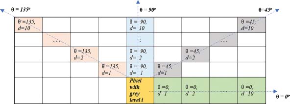
Figure 3: Representation of angular orientation θ and distances (1<= d<=0) between the pixel of grey level i and other pixels of interest
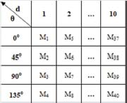
Figure 4: Arrangement of matrices covering four angular directions for ten distances (1 to 10)
Homogeneity, entropy, contrast and correlation are computed for these matrices which are summarized below.
Contrast:
It is local variation in an image that is calculated as the difference between the highest and lowest values of a given set of pixels. Contrast is given by:
Homogeneity:
It is also known as Inverse Difference Moment. It is an inverse distance difference, which is a local change in image texture. Its value decreases when most of the image elements are the same. Homogeneity is given as:
Entropy:
It is the amount of information in an image. If the image is not textually uniform, then its value is large. Also, it is strongly but inversely correlated to energy. Entropy is given by:
Correlation:
It is a linear dependency of gray tone in the image. Correlation is given
Here, σr ≠ 0, σc, and mr and mc are defined in equation 7 and 8.
From the arrangement of GLCM’s represented in figure 4, for each aforesaid four parameters, column/distance wise mean and variance are computed. Here, the size of computed means is of size 1x1 each. The size of variance of homogeneity as well as of variance of entropy is1x1 each, whereas it is 8x1 for both; variance of correlation and contrast. So, when computed at single distance, these means and variances are merged to form a feature vector of size 22x1. Further, when computed at ten different distances, the size of final GLCM feature vector becomes 220.
LBP
LBP features as suggested by authors in (Ojala et al., 1996) assigns a code for each pixel depending on its eight surrounded pixels' grey levels. A 3*3 mask is convolved through the image, and for each pixel, an LBP value is computed using equation 9.
Where, ic and in represent the intensity values of central pixel Pc and one of eight neighbors of Pc respectively as shown in figure 5. Further function s() is defined as:
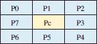
Figure 5: Central pixel Pc and its eight neighbors
For each prepared dataset image, the size of LBP feature vector is 59. When deep and texture features are merged, the size of final formulated FV becomes 4375.
3. Experimental results
Simulation work has been carried out using Matlab-R2020b (64 bit) version on intel i5-5200U processor of 2.2GHz system having 8GB of RAM. MIAS database is preprocessed and enlarged using the image augmentation technique. In this proposed work, the final feature vector (FFV) of length 4375 is created by merging features extracted from the modified DCNN using the TL technique with texture features extracted from GLCM and LBP. This FFV is given as input to various classifiers to measure their performance in terms of accuracy using k-fold (k=5 has been taken) cross-validation approach as shown in table 3. On the basis of value of k, the data set is divided randomly into 5 sets of equal size folds. Out of these 5 folds, random 4 folds are chosen for training purpose and the remaining fold is used for testing purpose. Compared to others, the Ensemble Boosted Tree (EBT) technique produces maximum classification accuracy of 98.8%.
Table 3: Accuracy measured for classification techniques on FFV
Method |
Accuracy |
Fine Tree |
95.00% |
Medium Tree |
89.90% |
Coarse Tree |
85.10% |
Coarse KNN |
83.90% |
Weighted KNN |
85.00% |
Ensemble Bagged Trees |
87.70% |
Ensemble Boosted Tree |
98.80% |
2576 is the total number of mammograms present in the augmented dataset. From these mammograms, 2160 belong to the benign class, whereas the remaining 416 to the malignant. Figure 6 represents the confusion matrix generated for the EBT technique on FFV. It shows 2160 is the number of true-positive (TP) cases, 385 true-negative (TN) cases, 31 false-positive (FP) cases and there is no false negative (FN) case. These parameters are used to measure the performance in respect of sensitivity, specificity and accuracy as defined in equation 11 to 13 respectively.
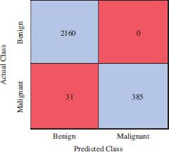
Figure 6: Confusion Matrix
The performance is also measured in terms of True Positive Rate (TPR), False Negative Rate (FNR) rate, Positive Prediction Values (PPV), and False Discovery Rates (FDR), which are explained in Table 4.
Table 4: Description and calculation formulas of TPR, FNR, PPV and FDR
Calculation for benign cases |
Calculation for malignant cases |
|
TPR: It is the proportion of correctly classified observations per actual class. |
||
FNR: It is the proportion of incorrectly classified observations per actual class. |
||
PPV: It is the proportion of correctly classified observations per classified class. |
||
FDR: It is the proportion of incorrectly classified observations per classified class. |
Using the confusion matrix of figure 6, computation of values of these four parameters are shown in figure 7.
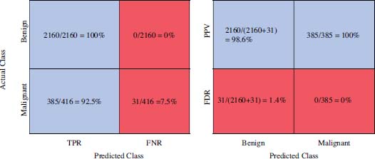
Figure 7: TPR, FNR, PPV, FDR calculation from confusion matrix
Performance comparison of the proposed model with other recent technologies in terms of sensitivity, specificity and accuracy is given in table 5 which shows its superiority over remaining models.
Table 5: Performance comparison of proposed work with recent techniques
Approach |
Sensitivity |
Specificity |
Accuracy |
Improving mass discrimination in mammogram-CAD system using texture information and super-resolution reconstruction (Boudraa et al., 2020) |
100% |
94.7% |
96.7% |
Automated diagnosis of breast cancer using parameter optimized kernel extreme learning machine (Mohanty et al., 2020) |
- |
- |
97.49% |
Deep learning and optimization algorithms for automatic breast cancer detection (Sha et al., 2020) |
96% |
93% |
92% |
Automatic Detection of Masses from Mammographic Images via Artificial Intelligence Techniques (Azlan et al., 2020) |
93.24% |
96.61% |
95.24% |
Breast Cancer: Tumor Detection in Mammogram Images Using Modified AlexNet Deep Convolution Neural Network (Omonigho et al., 2020) |
- |
- |
95.70% |
Multi-view feature fusion based four views model for mammogram classification using convolutional neural network (Khan et al., 2019) |
96.31% |
90.47% |
93.73% |
Proposed Method |
100% |
92.55% |
98.8% |
To measure the classifier’s performance, in addition to other methods described in this section, Receiver Operating Characteristic (ROC) curve can also be used. It represents the relationship between TPR and FPR. For the EBT classifier ROC curve are shown in figure 8(a) and figure 8(b). In ROC curve x and y axis represents the FPR and TPR of the classifier. In ROC curve as shown in figure 8 marked points represents the value pair of FPR and TPR. In figure 8(a), FPR value of 0.07 indicates that EBT classifier assigned 7% of the observation incorrectly to the positive class (benign), and TPR value of 1.0 indicates it assigned 100% of the observations correctly fore that it correctly to the positive class (benign). For malignant as true class, as shown in figure 8(b), the values of FPR and TPR are 0.0 and 0.93 respectively.
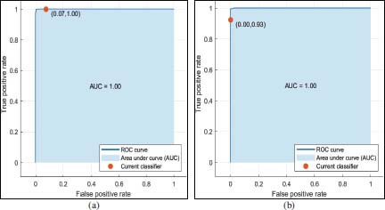
Figure 8: Representation of relationship between FPR and TPR using ROC curve for benign and malignant classes in figure 8(a) and figure (b) respectively
4. Conclusion and future scope
An automated breast cancer detection using mammogram images has been presented in this manuscript. MIAS images are processed through median filter and gaussian filter which is followed by segmentation and cropping to remove noise and unwanted regions. The preprocessed dataset is enhanced using the augmentation process to improve the classifier's training and testing quality. Combining texture (GLCM and LBP) features with those extracted from modified DCNN provided a good quality feature vector. Its performance has been evaluated over a number of classifiers, but the Ensemble Boosted Tree classifier gives maximum accuracy of 98.8%. Moreover, in terms of sensitivity and specificity, the same classifier produces 100% and 92.55% respectively using suggested feature set. In terms of performance, the proposed method is competitive to others. It can be used to fully automate pre-screening techniques, strengthening radiologist decisions, and prioritizing images for their subsequent assessment.
From future point of view, this approach can also be extended to classify mammogram images into three or more classes also. The performance of this approach can also be tested to detect masses from histopathology images, or other body part’s scanned images. After modification, it can also be investigated on 3-dimensional ultrasound images or digital breast tomosynthesis. With a choice to keep or discard used techniques, new techniques may be included in this multi-stage process as per requirement.
5. Acknowledgement
Authors would like to thank to Government of India for Visveswaraya Fellowship scheme for research under which this work has been carried out. Authors are also thankful for the valuable suggestions given by the reviewers which have been successfully incorporated.
References
Azlan, N. A. N., Lu, C. K., Elamvazuthi, I., & Tang, T. B. (2020). Automatic detection of masses from mammographic images via artificial intelligence techniques. IEEE Sensors Journal, 20(21), 13094-13102.
Boudraa, S., Melouah, A., & Merouani, H. F. (2020). Improving mass discrimination in mammogram-CAD system using texture information and super-resolution reconstruction. Evolving Systems, 11(4), 697-706.
Dibden A, Offman J, Duffy SW, Gabe R. Worldwide Review and Meta-Analysis of Cohort Studies Measuring the Effect of Mammography Screening Programmes on Incidence-Based Breast Cancer Mortality. Cancers. 2020; 12(4):976.
Haralick, R. M., Shanmugam, K., & Dinstein, I. H. (1973). Textural features for image classification. IEEE Transactions on systems, man, and cybernetics, (6), 610-621.
Khan, H. N., Shahid, A. R., Raza, B., Dar, A. H., & Alquhayz, H. (2019). Multi-view feature fusion based four views model for mammogram classification using convolutional neural network. IEEE Access, 7, 165724-165733.
Ko, S., & Lee, Y. (1998). Adaptive center weighted median filter. IEEE Transactions on Circuits and Systems, 38(9), 984-993.
Krizhevsky, A., Sutskever, I., & Hinton, G. E. (2012). Imagenet classification with deep convolutional neural networks. Advances in neural information processing systems, 25, 1097-1105.
Mathur, P., Sathishkumar, K., Chaturvedi, M., Das, P., Sudarshan, K. L., Santhappan, S., ... & ICMR-NCDIR-NCRP Investigator Group. (2020). Cancer statistics, 2020: report from national cancer registry programme, India. JCO Global Oncology, 6, 1063-1075.
Mohanty, F., Rup, S., & Dash, B. (2020). Automated diagnosis of breast cancer using parameter optimized kernel extreme learning machine. Biomedical Signal Processing and Control, 62, 102108.13
Nair, Vinod, and Geoffrey E. Hinton. «Rectified linear units improve restricted boltzmann machines». In Proceedings of the 27th international conference on machine learning (ICML-10), pp. 807-814. 2010.
Ojala, T., Pietikäinen, M., & Harwood, D. (1996). A comparative study of texture measures with classification based on featured distributions. Pattern recognition, 29(1), 51-59.
Omonigho, E. L., David, M., Adejo, A., & Aliyu, S. (2020, March). Breast Cancer: Tumor Detection in Mammogram Images Using Modified AlexNet Deep Convolution Neural Network. In 2020 International Conference in Mathematics, Computer Engineering and Computer Science (ICMCECS) (pp. 1-6). IEEE.
Otsu N. A threshold selection method from gray-level histogram. IEEE Transactions on System Man and Cybemetic. 9(1): 62-66, 1979.
Sannasi Chakravarthy, S. R., & Rajaguru, H. (2020). Detection and classification of microcalcification from digital mammograms with firefly algorithm, extreme learning machine and non‐linear regression models: A comparison. International Journal of Imaging Systems and Technology, 30(1), 126-146.
Sha, Z., Hu, L., & Rouyendegh, B. D. (2020). Deep learning and optimization algorithms for automatic breast cancer detection. International Journal of Imaging Systems and Technology, 30(2), 495-506.
Sharma, B. P., & Purwar, R. K. (2020, July). Dual Thresholding based Breast cancer detection in Mammograms. Fourth IEEE World Conference on Smart Trends in Systems, Security and Sustainability (WorldS4) (pp. 589-592).
Song, R., Li, T., & Wang, Y. (2020). Mammographic Classification Based on XGBoost and DCNN With Multi Features. IEEE Access, 8, 75011-75021.
Srivastava, N., Hinton, G., Krizhevsky, A., Sutskever, I., & Salakhutdinov, R. (2014). Dropout: a simple way to prevent neural networks from overfitting. The journal of machine learning research, 15(1), 1929-1958.
Suckling J, Parker J, Dance D, Astley S, Hutt I, Boggis C, et al. The mammographic image analysis society digital mammogram database. Exerpta Medica. 1994; 1069:375–8
Sung, H, Ferlay, J, Siegel, RL, Laversanne, M, Soerjomataram, I, Jemal, A, Bray, F. Global Cancer Statistics 2020: GLOBOCAN Estimates of Incidence and Mortality Worldwide for 36 Cancers in 185 Countries. CA Cancer J Clin. 2020.
Young, I. T., & van Vliet, L. J. (1995). Recursive implementation of the Gaussian filter. Signal Processing, 44(2), 139–151. doi:10.1016/0165-1684(95)00020-e.
Zhang, X., Zhang, Y., Han, E. Y., Jacobs, N., Han, Q., Wang, X., & Liu, J. (2018). Classification of whole mammogram and tomosynthesis images using deep convolutional neural networks. IEEE transactions on nanobioscience, 17(3), 237-242.