
Regular Issue, Vol. 10 N. 3 (2021), 293-305
eISSN: 2255-2863
DOI: https://doi.org/10.14201/ADCAIJ2021103293305
|
ADCAIJ: Advances in Distributed Computing and Artificial Intelligence Journal
Regular Issue, Vol. 10 N. 3 (2021), 293-305 eISSN: 2255-2863 DOI: https://doi.org/10.14201/ADCAIJ2021103293305 |
Projects Distribution Algorithms for Regional Development
Mahdi Jemmali
Department of Computer Science and Information, College of science at Zulfi, Majmaah University, AL-Majmaah 11952, Saudi Arabia
MARS Laboratory, University of Sousse, Tunisia
Department of Computer Science, Higher institute of computer Science and mathematics, University of Monastir, Monastir, 5000, Tunisia
ABSTRACT
This paper aims to find an efficient method to assign different projects to several regions seeking an equity distribution of the expected revenue of projects. The solutions to this problem are discussed in this paper. For this work, the constraint is to suppose that all regions have the same socio-economic proprieties. Given a set of regions and a set of projects. Each project is expected to elaborate a fixed revenue. The goal of this paper is to minimize the summation of the total difference between the total revenues of each region and the minimum total revenue assigned to regions. An appropriate schedule of projects is the schedule that ensures an equitable distribution of the total revenues between regions. A load balancing of the total expected revenue in each region must be ensured. In this paper, we give a mathematical formulation of the objective function and propose several algorithms to solve the studied problem. An experimental result is presented to discuss the comparison between all implemented algorithms.
KEYWORDS
Approximate solution; Regional development; Project distribution; Algorithms
1. Introduction
This research is based on the equity distribution of new projects making it possible to return financial gains to the regions. These financial gains participate in the first place in the development of the region concerned. For this, an approach must be established that guarantees the equity distribution of projects to ensure a balance in terms of income between regions. This approach must imperatively seek to minimize the gap in terms of revenue returned by projects. Otherwise, a remarkable gap can lead to a bad decision.
The studied problem can be described as follows. Assume that we have different projects, having each an expected revenue, to be scheduled to different regions. Each project is characterized by its proper expected revenue. The constraint of the studied problem is to consider all regions have the same socio-economic characterization. The objective is to find a schedule that can give a minimum revenue gap between regions. This problem is proposed for the first time in the literature review (Jemmali, 2019a). In the latter work, the author proposed a mathematical model to present the objective of the research. Indeed, this medialization is based on the minimization of the total gap between the total revenue in each region and the minimum assigned revenue. In addition, the author developed three approximate solutions. The first one is based essentially on the randomization method. The second one is based on the iterative method. The third one is based on the change of the probabilistic values.
Similar work is developed in (Jemmali, 2019b). In this latter work, the author presents the problem with another objective function which is the minimization of the maximum revenue assigned. Several heuristics were proposed based essentially on the dispatching rules and the multi-fit approach. An experimental result was discussed to perform the proposed heuristics.
In (Alharbi & Jemmali, 2020), the authors proposed lower bounds, approximates solutions, and a branch and bound method for the project distribution. In this latter work, the objective function is different comparing with the objective functions proposed in (Jemmali, 2019a) and (Jemmali, 2019b). Indeed, the objective function proposed in the recent work is the minimization of the sum of the difference between the maximum revenue and the revenue of each region.
Recently, the author of (Jemmali, 2021) developed an optimal solution for the budget assignment problem. Several lower bounds and upper bounds were developed in the latter research work to be used in the branch and bound algorithm.
Several research works treated the load balancing on different domains. Indeed, in (Alquhayz et al., 2020) the load balancing method is applied to the used spaces of storage supports. Several heuristics was developed in this latter research-based essentially o the swapping between the different dispatching rules. In the network domain, equity distribution is developed to ensure the equity transmission of the data through a network (Jemmali & Alquhayz, 2020).
Another domain to apply the load balancing is the gas turbine aircraft engine problem (Jemmali et al., 2019b) and (Jemmali et al., 2019a).
In (Haouari & Jemmali, 2008), authors proposed several solutions related to the problem seeking to maximize the minimum completion time on identical parallel machines. An exact solution was developed. An enhancement of the solutions found in the latter work was proposed in (Walter et al., 2017).
Several types of research aim to find a better resources distribution (de Sena et al., 2013), (Ho et al., 2012), (Ospina López, 2019), (Yeo et al., 2021), (Research Group on Innovative Development of Public Services in Beijing, 2021) and (Khanizad & Montazer, 2021). Other applications of the resource distribution can be cited (Tseng et al., 2020) (Rudek & Heppner, 2020) (Kavoosi et al., 2020) and (Ehmann et al., 2021).
On other hand, the load balancing algorithms were used in several domains (Arulkumar & Bhalaji, 2021), (Gupta et al., 2020), (Tapale et al., 2021), (Priya et al., 2019), (Ebadifard & Babamir, 2018), and (Li & Wu, 2019).
A resource-constrained project scheduling was proposed in (Alcaraz & Maroto, 2001). In this latter research, the genetic algorithm gave the best result. In (Maguluri et al., 2014), the authors proposed a stochastic model of cloud computing using the model where the resource allocation problem can be separated into a routing or load balancing problem and a scheduling problem. A resource allocation problem was studied applied to a fog-cloud environment (Naha et al., 2020).
In this research, we propose the mathematical formulation of the problem and several developed heuristics to solve the studied problem. The experimental results show the performance of the proposed heuristics.
The rest of this paper is organized as follows. The second section is reserved for the problem description. Section 3 consist to propose the heuristics for solving the studied problem. The experimental results are reserved in Section 4. Section 5 is for the conclusions.
2. Motivation and justification
This research work can be described as follows. Assume that there are different projects characterized by an expected revenue. These projects must be assigned to regions. In a development country it is important to seek the equity distribution of the expected revenue to regions. This means we search the equity distribution of projects to regions. The objective is to find a schedule that can give a minimum revenue gap between regions. To reach this objective we propose a mathematical modeling and several proposed heuristics to solve the studied problem.
3. Problem description
In a country, there are several regions. The objective is to promote regional development in this country. Several projects with expected revenues are proposed to be applied to nℜ regions. The number of projects is denoted by npr. The expected revenue of each project Ppr with pr = {1,…,npr} is denoted by rpr. The set of projects is denoted by P. The cumulative expected revenue due to the assignment of the project pr is denoted by Crpr. After finishing the assignment of all projects to regions, the total revenue on each region is denoted by Tℜ with ℜ = {1,…, nℜ}. The minimum (maximum) total obtained revenues on a region after finishing scheduling is denoted by Tmin(Tmax). The following example describes the studied problem with all the above notations.
Example 1
Assume that we have the number of projects npr = 6. The number of regions that we must schedule the 6 projects is 2 (nℜ = 2). The revenue of each project is given in Table 1.
Table 1. Distribution of revenue for each project.
pr |
1 |
2 |
3 |
4 |
5 |
6 |
rpr |
50 |
135 |
250 |
170 |
80 |
75 |
Now, we apply any algorithm to distribute the projects in Table 1 to the regions. Applying the shortest processing time rule, the result is depicted in Figure 1. This latter figure shows that projects {1,4,5} are assigned to region 1 and projects {2,3,6} are assigned to region 2.
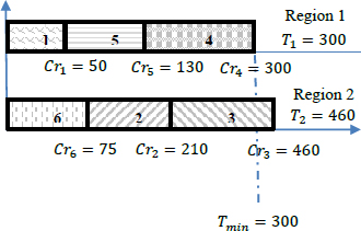
Figure 1. Schedule for 6-projects and 2-regions
Based on Figure 1, region 1 has a total expected revenue of 300. However, region 2 has a total expected revenue of 460. Consequently, the expected revenue gap between region 1 and region 2 is T2 − Tmin = 160. In this paper, we search to reduce the obtained gap between regions. Indeed, for this example, we try to find a schedule more efficient with a gap of less than 160.
Now, in general, if we have several regions we have to fix an indicator through it we can calculate the efficiency of the algorithm that seeking the fair distribution. Equation (1), represent the gap that must be minimized to ensure equity.
Proposition 1
The gap gr in Equation 1 can be written as follows.
4. Proposed algorithms
The first algorithm is the longest project revenue which is based on the dispatching rule. Also, the smallest project revenue is a dispatching rule algorithm. For the third algorithm, we apply a mixture method between the first and the second rules. The fourth algorithm is another variant of the mixture. The last algorithm is based on the probabilistic and randomization method.
We denoted by (L) the function that returns the project that has the longest revenue from list L. However, ST(L) is the function that returns the project that has the smallest revenue from list L. We denoted by Schd(−) the function that applied on a project and schedule it on the region that having the minimum cumulative revenue.
4.1. Longest project revenue (LPR)
This algorithm is based on the following idea. The first step is to sort all project revenue in decreasing order. After that, we schedule the project that has the longest revenue in the region that having the minimum cumulative revenue and so on until finish all projects.
4.2. Smallest project revenue (SPR)
This algorithm is based on the following idea. The first step is to sort all project revenue on the increasing order. After that, we schedule the project that has the smallest revenue in the region that having the minimum cumulative revenue and so on until finish all projects.
4.3. Longest-smallest- half-mixed algorithm (LSHM)
This algorithm is based on the mixed choice of the selection of projects. Indeed, half of the projects will be scheduled applying the longest revenue first on region that having the minimum cumulative revenue. After that, the second half of projects will be scheduled applying the smallest revenue first. The instructions of the heuristic longest-smallest- half-mixed algorithm are illustrated in Algorithm 1. In Algorithm 1, the variable pr is initialized to npr and the list L is initialized to P. Firstly, we search the project that having the longest revenue applying the function LT(−). The value returned by the latter function is assigned to variable Pc. The latter variable contain the index of the project which will be scheduled on regions calling the function Schd(−). This procedure will be repeated until reaching . After that, the half of projects are scheduled. For the remaining projects we apply the same idea of the scheduling. Indeed, for each iteration of pr, instead of selecting the project that having the longest revenue from the remaining list, we select the project that having the smallest revenue. We schedule the selected project, updating the list L and so on until finishing all projects from L.
Algorithm 1: Longest-Smallest half-mixed algorithm (LSHM) |
|
1 |
Set pr = npr, L = P |
2 |
while () do |
3 |
Pc = LT(L) |
4 |
Schd(Pc) |
5 |
L = L\Pc |
6 |
pr −− |
7 |
End while |
8 |
pr = 1 |
9 |
while () do |
10 |
Pc = ST(L) |
11 |
Schd(Pc) |
12 |
L = L\Pc |
13 |
pr ++ |
14 |
End while |
15 |
Calculate gr |
16 |
Return gr |
Algorithm 2: Swapping longest-smallest algorithm (SLS) |
|
1 |
Set pr = 1, L = P |
2 |
while (pr ≤ npr) do |
3 |
if (Mod()=1) then |
4 |
Pc = LT (L) |
5 |
else |
6 |
Pc = ST (L) |
7 |
end if |
8 |
Schd (Pc) |
9 |
L = L\Pc |
10 |
pr ++ |
11 |
end while |
12 |
Calculate gr |
13 |
Return gr |
4.4. Swapping longest-smallest algorithm (SLS)
For this algorithm, we adopt to choose among all projects once the project having the longest revenue and once the project having the smallest revenue. Indeed, a variable pr is declared and initialized to 1. For each iteration in the algorithm, a test of parity is executed. Thus, if pr is even, we call LT(−) on the remaining projects. The returned value of LT(−) containing the index of the selected project. The selected project will be scheduled on the region that having the minimum cumulative revenue calling the function Schd(−). On the other hand, if pr is odd, we call ST(−) on the remaining projects. The returned value of ST(−) containing the index of the selected project. The selected project will be scheduled on the region that having the minimum cumulative revenue calling the function Schd(−).
The instruction of the heuristic swapping longest-smallest algorithm are illustrated in Algorithm 2.
4.5. Randomized Longest project revenue algorithm (RLPR)
This algorithm is based on the fact that instead to choose the project that has the longest revenue, we choose among the two projects that have the longest revenues with probability β. Indeed, between the selected two projects one will be assigned to a region that having the minimum cumulative revenue. In practice a number r will be generated randomly between [1-100]. If r<30 then we select the first project that having the longest revenue else we select the second project that having the longest revenue. We iterate the algorithm several times and we pick up the best solution. In practice, the number of repetitions is fixed to 1000.
5. Experimental results
In this section, generate different classes of instances to make a comparison with all developed algorithms in terms of gap and time. All algorithms developed in this research are implemented with Microsoft Visual C++ (Version 2013). The results are obtained after running all programs related to the proposed algorithms on an Intel(R) Core(TM) i5-3337U CPU @ 1.8 GHz and 8 GB RAM. The operating system utilized throughout the work is windows 10 with 64 bits.
The developed algorithms were compared applying 5 categories of instances. These categories were generated as presented in (Jemmali, 2019b)
The revenue of project rpr is generated using the normal distribution and the uniform distribution. The choice of these distributions is fixed by the following classes:
• Class 1: generate the project revenue (rpr) according to U[30,100].
• Class 2: generate the project revenue (rpr) according to U[50,300].
• Class 3: generate the project revenue (rpr) according to U[200,500].
• Class 4: generate the project revenue (rpr) according to N[50,150].
• Class 5: generate the project revenue (rpr) according to N[25,500].
with U[x,y] is the uniform distribution in [x,y] and N[x,y] is the normal distribution. The generation of an instance is dependent on the choice of npr, nre, and Class. The pair (npr, nre) can have several values. In fact, we adopt the values given in Table 2.
Table 2. The npr and nre values
npr |
nre |
10 |
2,3,5 |
25,50 |
2,3,5,10,15 |
100,250 |
3,5,10,15,25,30 |
300,500 |
10,15,30,50 |
Table 2 shows that the total number of instances is 1650. Different indicators are proposed in this paper to illustrate the comparison between the developed algorithms:
• Lm best-obtained value after executing all algorithms.
• L value of the studied algorithm.
• .
• Time average running time in seconds. The notation of “-“ is putted when the running time is less than 0.001 s.
• Per percentage of instances satisfying Lm = L.
Table 3 represents the comparison of the percentage and time for all algorithms. From this table, we can deduce that RLPR is the best algorithm with 94.3% comparing with others in an average time of 0.050s.
Table 3. Overall comparison of Per and Time for all algorithms
|
LPR |
SPR |
LSHM |
SLS |
RLPR |
Per |
19.5% |
0.0% |
4.9% |
5.8% |
94.3% |
Time |
- |
- |
- |
- |
0.050 |
Table 4. Variation of G according to npr
npr |
LPR |
SPR |
LSHM |
SLS |
RLPR |
10 |
0.41 |
0.77 |
0.70 |
0.65 |
0.00 |
25 |
0.45 |
0.72 |
0.59 |
0.60 |
0.00 |
50 |
0.56 |
0.88 |
0.81 |
0.74 |
0.00 |
100 |
0.37 |
0.79 |
0.63 |
0.73 |
0.01 |
250 |
0.29 |
0.81 |
0.68 |
0.75 |
0.01 |
300 |
0.30 |
0.91 |
0.85 |
0.89 |
0.00 |
500 |
0.14 |
0.78 |
0.61 |
0.71 |
0.02 |
Table 5. Variation of G according to nℜ
nℜ |
LPR |
SPR |
LSHM |
SLS |
RLPR |
2 |
0.78 |
0.94 |
0.93 |
0.66 |
0.00 |
3 |
0.56 |
0.76 |
0.65 |
0.70 |
0.00 |
5 |
0.49 |
0.91 |
0.88 |
0.91 |
0.00 |
10 |
0.37 |
0.88 |
0.81 |
0.84 |
0.00 |
15 |
0.12 |
0.65 |
0.40 |
0.51 |
0.02 |
25 |
0.32 |
0.89 |
0.82 |
0.87 |
0.00 |
30 |
0.11 |
0.69 |
0.50 |
0.60 |
0.02 |
50 |
0.16 |
0.86 |
0.77 |
0.84 |
0.00 |
Table 4 shows that the maximum G value is obtained 0.88 for algorithm SPR when npr = 50. The algorithm that having the minimum average gap is RLPR.
The variation of G according to nℜ is given in Table 5.
Table 6 shows the variation of the gap according to classes. From this table, we can observe that for algorithm RLPR classes 2 and 4 the gap is 0 but for other classes, the gap is 0.01. However, for SLS, LSHM, and SPR the minimum average gap is obtained for class 5.
Tables 7,8 and 9 shows the variation of time according to npr, nℜ and Class, respectively.
Table 9 shows that the maximum running time of 0.53 s is obtained for algorithm RLPR and for Class 3.
Table 10 presents the variation of G according to nℜ and npr.
Table 6. Variation of G according to Class
Class |
LPR |
SPR |
LSHM |
SLS |
RLPR |
1 |
0.29 |
0.86 |
0.71 |
0.77 |
0.01 |
2 |
0.41 |
0.91 |
0.85 |
0.85 |
0.00 |
3 |
0.35 |
0.83 |
0.67 |
0.75 |
0.01 |
4 |
0.47 |
0.86 |
0.75 |
0.74 |
0.00 |
5 |
0.30 |
0.57 |
0.49 |
0.52 |
0.01 |
Table 7. Variation of Time according to npr
npr |
LPR |
SPR |
LSHM |
SLS |
RLPR |
10 |
- |
- |
- |
- |
0.003 |
25 |
- |
- |
- |
- |
0.006 |
50 |
- |
- |
- |
- |
0.010 |
100 |
- |
- |
- |
- |
0.026 |
250 |
- |
- |
- |
- |
0.064 |
300 |
- |
- |
- |
- |
0.097 |
500 |
- |
- |
- |
- |
0.161 |
Table 8. Variation of Time according to nℜ
nℜ |
LPR |
SPR |
LSHM |
SLS |
RLPR |
2 |
- |
- |
- |
- |
0.005 |
3 |
- |
- |
- |
- |
0.016 |
5 |
- |
- |
- |
- |
0.017 |
10 |
- |
- |
- |
- |
0.050 |
15 |
- |
- |
- |
- |
0.056 |
25 |
- |
- |
- |
- |
0.055 |
30 |
- |
- |
- |
- |
0.097 |
50 |
- |
- |
- |
- |
0.172 |
Table 9. Variation of Time according to Class
Class |
LPR |
SPR |
LSHM |
SLS |
RLPR |
1 |
- |
- |
- |
- |
0.049 |
2 |
- |
- |
- |
- |
0.052 |
3 |
- |
- |
- |
- |
0.053 |
4 |
- |
- |
- |
- |
0.050 |
5 |
- |
- |
- |
- |
0.048 |
Table 10. Variation of G according to nℜ and npr
npr |
nℜ |
LPR |
SPR |
LSHM |
SLS |
RLPR |
10 |
2 |
0.78 |
0.97 |
0.97 |
0.68 |
0.00 |
3 |
0.45 |
0.68 |
0.53 |
0.59 |
0.00 |
|
5 |
0.00 |
0.67 |
0.61 |
0.68 |
0.00 |
|
25 |
2 |
0.83 |
0.85 |
0.82 |
0.85 |
0.00 |
3 |
0.60 |
0.77 |
0.74 |
0.70 |
0.00 |
|
5 |
0.68 |
0.95 |
0.95 |
0.94 |
0.00 |
|
10 |
0.13 |
0.54 |
0.30 |
0.39 |
0.00 |
|
15 |
0.00 |
0.47 |
0.16 |
0.13 |
0.00 |
|
50 |
2 |
0.72 |
0.99 |
0.99 |
0.46 |
0.00 |
3 |
0.82 |
0.86 |
0.82 |
0.79 |
0.00 |
|
5 |
0.64 |
0.97 |
0.95 |
0.97 |
0.00 |
|
10 |
0.49 |
0.93 |
0.91 |
0.91 |
0.01 |
|
15 |
0.12 |
0.63 |
0.38 |
0.56 |
0.00 |
|
100 |
3 |
0.57 |
0.77 |
0.63 |
0.73 |
0.00 |
5 |
0.62 |
0.98 |
0.96 |
0.97 |
0.00 |
|
10 |
0.49 |
0.94 |
0.89 |
0.92 |
0.00 |
|
15 |
0.09 |
0.56 |
0.18 |
0.34 |
0.04 |
|
25 |
0.35 |
0.88 |
0.81 |
0.86 |
0.00 |
|
30 |
0.08 |
0.61 |
0.33 |
0.57 |
0.00 |
|
250 |
3 |
0.38 |
0.73 |
0.52 |
0.67 |
0.00 |
5 |
0.50 |
0.98 |
0.96 |
0.98 |
0.00 |
|
10 |
0.42 |
0.95 |
0.93 |
0.94 |
0.00 |
|
15 |
0.11 |
0.62 |
0.28 |
0.41 |
0.08 |
|
25 |
0.30 |
0.90 |
0.83 |
0.89 |
0.00 |
|
30 |
0.04 |
0.66 |
0.57 |
0.60 |
0.00 |
|
300 |
10 |
0.41 |
0.96 |
0.93 |
0.95 |
0.00 |
15 |
0.36 |
0.94 |
0.89 |
0.94 |
0.00 |
|
30 |
0.26 |
0.89 |
0.82 |
0.85 |
0.01 |
|
50 |
0.17 |
0.86 |
0.76 |
0.83 |
0.00 |
|
500 |
10 |
0.29 |
0.96 |
0.92 |
0.95 |
0.00 |
15 |
0.05 |
0.71 |
0.49 |
0.67 |
0.00 |
|
30 |
0.07 |
0.60 |
0.26 |
0.39 |
0.06 |
|
50 |
0.15 |
0.86 |
0.77 |
0.84 |
0.00 |
6. Conclusion
In this paper, we treated the problem of the fair distribution of several projects having each an expected revenue to be scheduled on different regions. The problem is strongly NP-hard. A mathematical formulation of the objective function is proposed in this paper to solve the studied problem. Several algorithms are developed and implemented to show the performance of the approach. The two first algorithms are based on the sorting rules. The two other algorithms are based on the swapping and mixture techniques. The last algorithm is based on the randomization and the probabilistic method. An experimental result is developed with 1650 instances to show the performance of the proposed algorithms. The comparison between the results returned by all algorithms proves that RLPR is the best algorithm comparing with others based on the gap indicator with a percentage of 94.3%. The average running time of the latter algorithm is 0.05 s. The best algorithm RLPR can be applied to solve the problem of the fair distribution of projects in a development country. This algorithm can be performed and enhanced using the genetic algorithm. The proposed algorithms can be used to solve other economic problems and to find an exact solution of the studied problem.
Acknowledgment
The authors would like to thank the Deanship of Scientific Research at Majmaah University for supporting this work under project no R-2021-145
7. References
Alcaraz, J., & Maroto, C. (2001). A robust genetic algorithm for resource allocation in project scheduling. Annals of operations Research, 102(1), 83-109.
Alharbi, M., & Jemmali, M. (2020). Algorithms for Investment Project Distribution on Regions. Computational Intelligence and Neuroscience, 2020.
Alquhayz, H., Jemmali, M., & Otoom, M. M. (2020). Dispatching-rule variants algorithms for used spaces of storage supports. Discrete Dynamics in Nature and Society, 2020.
Arulkumar, V., & Bhalaji, N. (2021). Performance analysis of nature inspired load balancing algorithm in cloud environment. Journal of Ambient Intelligence and Humanized Computing, 12(3), 3735-3742.
de Sena, D. C., Soares, E. F., de Paiva, I. V. L., & do Carmo, B. B. T. (2013). Queue balancing of load and expedition service in acement industry in Brazil. Independent Journal of Management & Production, 4(2), 452-462.
Ebadifard, F., & Babamir, S. M. (2018). A PSO-based task scheduling algorithm improved using a load-balancing technique for the cloud computing environment. Concurrency and Computation: Practice and Experience, 30(12), e4368.
Ehmann, M. R., Zink, E. K., Levin, A. B., Suarez, J. I., Belcher, H. M., Biddison, E. L. D., Doberman, D. J., D’Souza, K., Fine, D. M., & Garibaldi, B. T. (2021). Operational recommendations for scarce resource allocation in a public health crisis. Chest, 159(3), 1076-1083.
Gupta, A., Bhadauria, H., & Singh, A. (2020). Load balancing based hyper heuristic algorithm for cloud task scheduling. Journal of Ambient Intelligence and Humanized Computing, 1-8.
Haouari, M., & Jemmali, M. (2008). Maximizing the minimum completion time on parallel machines. 4OR, 6(4), 375-392.
Ho, G. T., Ip, W., Lee, C. K., & Mou, W. (2012). Customer grouping for better resources allocation using GA based clustering technique. Expert Systems with Applications, 39(2), 1979-1987.
Jemmali, M. (2019a). Approximate solutions for the projects revenues assignment problem. Communications in Mathematics and Applications, 10(3), 653-658.
Jemmali, M. (2019b). Budgets balancing algorithms for the projects assignment. International Journal of Advanced Computer Science and Applications (IJACSA), 10(11), 574-578.
Jemmali, M. (2021). An optimal solution for the budgets assignment problem. RAIRO: Recherche Opérationnelle, 55, 873.
Jemmali, M., & Alquhayz, H. (2020). Equity data distribution algorithms on identical routers. International Conference on Innovative Computing and Communications,
Jemmali, M., Melhim, L. K. B., & Alharbi, M. (2019a). Randomized-variants lower bounds for gas turbines aircraft engines. World Congress on Global Optimization,
Jemmali, M., Melhim, L. K. B., Alharbi, S. O. B., & Bajahzar, A. S. (2019b). Lower bounds for gas turbines aircraft engines. Communications in Mathematics and Applications, 10(3), 637-642.
Kavoosi, M., Dulebenets, M. A., Pasha, J., Abioye, O. F., Moses, R., Sobanjo, J., & Ozguven, E. E. (2020). Development of algorithms for effective resource allocation among highway–rail grade crossings: a case study for the State of Florida. Energies, 13(6), 1419.
Khanizad, R., & Montazer, G. A. (2021). A model for optimal allocation of human resources based on the operational performance of organisational units by multi-agent systems. International Journal of Operational Research, 40(1), 32-51.
Li, G., & Wu, Z. (2019). Ant colony optimization task scheduling algorithm for SWIM based on load balancing. Future Internet, 11(4), 90.
Maguluri, S. T., Srikant, R., & Ying, L. (2014). Heavy traffic optimal resource allocation algorithms for cloud computing clusters. Performance Evaluation, 81, 20-39.
Naha, R. K., Garg, S., Chan, A., & Battula, S. K. (2020). Deadline-based dynamic resource allocation and provisioning algorithms in fog-cloud environment. Future Generation Computer Systems, 104, 131-141.
Ospina López, J. P. (2019). A omputational justice model for resources distribution in Ad Hoc Networks.
Priya, V., Kumar, C. S., & Kannan, R. (2019). Resource scheduling algorithm with load balancing for cloud service provisioning. Applied Soft Computing, 76, 416-424.
Research Group on Innovative Development of Public Services in Beijing, I. o. M. S., Beijing Academy of Social Sciences zhaoran@ ssap. cn. (2021). More Balanced Distribution and Overall Quality Improvement of Public Services in Beijing. Analysis of the Development of Beijing, 2019, 99-126.
Rudek, R., & Heppner, I. (2020). Efficient algorithms for discrete resource allocation problems under degressively proportional constraints. Expert Systems with Applications, 149, 113293.
Tapale, M. T., Goudar, R., & Birje, M. N. (2021). Load Balancing Using Firefly Approach. In Progress in Advanced Computing and Intelligent Engineering (pp. 483-492). Springer.
Tseng, J.-H., Chen, Y.-F., & Wang, C.-L. (2020). User selection and resource allocation algorithms for multicarrier NOMA systems on downlink beamforming. IEEE Access, 8, 59211-59224.
Walter, R., Wirth, M., & Lawrinenko, A. (2017). Improved approaches to the exact solution of the machine covering problem. Journal of Scheduling, 20(2), 147-164.
Yeo, S., Naing, Y., Kim, T., & Oh, S. (2021). Achieving Balanced Load Distribution with Reinforcement Learning-Based Switch Migration in Distributed SDN Controllers. Electronics, 10(2), 162.