
Regular Issue, Vol. 10 N. 3 (2021), 241-266
eISSN: 2255-2863
DOI: https://doi.org/10.14201/ADCAIJ2021103241266
|
ADCAIJ: Advances in Distributed Computing and Artificial Intelligence Journal
Regular Issue, Vol. 10 N. 3 (2021), 241-266 eISSN: 2255-2863 DOI: https://doi.org/10.14201/ADCAIJ2021103241266 |
Advance Approach for Detection of DNS Tunneling Attack from Network Packets Using Deep Learning Algorithms
Gopal Sakarkar1, Mahesh Kumar H Kolekar2, Ketan Paithankar3, Gaurav Patil4, Prateek Dutta4, Ruchi Chaturvedi4, Shivam Kumar4
[1] Assistant Professor AIML, G H Raisoni College of Engineering, Nagpur, Maharashtra
[2] Associate Professor, IIT Patna
[3] CTO Konverge.ai, Nagpur, M.H
[4] Student, G H Raisoni College of Engineering, Nagpur, Maharashtra
(g.sakarkar@gmail.com, mahesh@iitp.ac.in, ketan@konverge.ai, gauravpatil22301@gmail.com, prateekdutta2001@gmail.com, rch432@gmail.com, sinhashivam22@gmail.com)
ABSTRACT
Domain Name System (DNS) is a protocol for converting numeric IP addresses of websites into a human-readable form. With the development of technology, to transfer information, a method like DNS tunneling is used which includes data encryption into DNS queries. The ability of the DNS tunneling method of transferring data attracts attackers to establish bidirectional communication with machines infected with malwares. This can lead to sending instructions in an obfuscated way or can lead to data exfiltration. Since firewalls and intrusion detection systems detect only specific types of tunneling, were as the Machine Learning Algorithms can analyze and predict based on previous data provided to it, it is being adopted by researchers to detect and predict the occurrence of DNS Tunneling. The identification of anomalies in Network packets can be done by using Natural Language Processing (NLP) technique. The experimental test accuracy showed that the feature extraction method in NLP for detecting DNS tunneling in network packets was found to be 98.42% on the generated Dataset. This paper makes a comparative study of 1 Dimensional Convolution Neural Network (1-D CNN), Simple Recurrent Neural Network (Simple RNN), Long Short-Term Memory (LSTM) algorithm, Gated Recurrent Unit (GRU) algorithm for detecting DNS Tunneling over the generated dataset. To detect this threat of DNS tunneling attack, good quality of the dataset is required. This paper also proposes the generation of a good quality dataset that contains network packets, by the recreation of DNS Tunneling attack using tool dnscat2. The Precision, recall and f1 score obtain for LSTM algorithm on 80:20 split was 99%, 98% and 98% respectively.
KEYWORDS
Text Classification, Machine Learning, NLP, LSTM,1-D CNN, RNN, GRU, DNS packet, Deep Learning, DNS Tunneling, Wireshark, dnscat2
1. Introduction
In just a few decades there was tremendous growth with the internet which was unpredictable at the time of its creation. At the time of creation, it connected small areas and it was not designed keeping security in mind. The modern Internet has inherited this lack of security in many ways. The Domain name System (DNS) system is the core part of the internet infrastructure made for name resolution, but during past years some approaches have been developed to use it for data transfer. They attract the hacker to exploit DNS to carry out attacks such as Distributed Denial of Service (DDoS) attacks, DNS spoofing, and DNS tunneling. DDoS Attack obstructs the network availability by overflowing the victim with a high volume of illegal traffic usurping its bandwidth, overburdening it to prevent valid traffic to get through [1]. DNS spoofing, also known as DNS cache poisoning attack, diverting traffic to another computer and returning an incorrect IP address, when the data is introduced into a Domain Name Server [2]. DNS tunneling is an attack that exploits the domain name protocol to bypass security gateways [3]. For this paper, we restricted we have focused on detecting DNS Tunneling attack.
The past few years have experienced a great rise and various researches were done in the field of Artificial Intelligence [4]. The importance of Artificial Intelligence in the detection of attack is playing a significant role [5]. Machine learning techniques focus on building a system model that enhances its performance based on previous results [6]. Alternatively, it can be said that systems based upon machine learning can manipulate execution strategies based upon new inputs [7]. In paper [8], authors proposed a system for detecting known and unknown Distributed Denial of Service (DDoS) Attacks using two different intrusion detection approaches i.e. anomaly-based distributed artificial neural networks (ANNs) and signature-based approach. In paper [9], researchers propose the use of a classification model based on an artificial recurrent neural network (RNN) and a deep learning approach for DNS spoofing detection. Various methods are proposed to detect DNS tunneling attacks using Machine learning and Deep learning Algorithm implementation. In paper [10], To detect DNS tunneling fast and accurately, this paper proposes a detection approach based on a Convolutional Neural Network (CNN) with a minimal architecture complexity. This paper [11], aims to provide a comparative study for three machine learning techniques including Support Vector Machine (SVM), Naive Bayes (NB), and J48, or so-called Decision Tree (DT) for DNS tunneling Detection. In paper [12], researchers propose a detection method based on deep learning models, which uses the DNS query payloads as predictive variables in the models with the approach of word embedding as a part of fitting the neural networks.
In this paper, we have generated a novel dataset containing network packets of DNS tunneling attacks and methods for detecting it using network packets. This paper used the network query payloads as predictive variables in the models. Our approach uses word embedding as a part of fitting the neural networks, which is a feature extraction method in natural language processing (NLP) on the generated DNS tunneling dataset. To achieve higher performance, we have made use of LSTM and GRU algorithms in our neural network. The paper also includes the comparative study between Simple RNN, 1-D CNN, LSTM, and GRU over the generated dataset.
1.1. Technical Concepts
Domain Name System represents a complex protocol running under an application layer of the International Organization for Standardization (ISO)/ Open System Interconnection (OSI) model. It is an application holding the database of Internet protocol (IP) addresses mapped to another hostname and it resolves the IP address to another domain name. DNS protocols redirect network traffic based on name and numeric addresses. Various attacks are targeting DNS such as cache poisoning, NXDomain & phantom domain attack, domain hijacking and redirection, data Exfiltration, and tunneling [13]. This attack can lead to common abuse cases such as malware command and control(C&C), creating a firewall bypass tunneling, Bypass Captive portal for paid wi-fi [14].
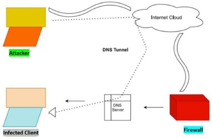
Figure 1: Working of DNS Tunneling attack
As shown in Fig. 1, the attacker first infects the DNS client with malware that opens a tunnel to the attacker's machine via a duplicate DNS server located in the client network area, thus passing the network firewall. HTTPS traffic can also be exchanged via a DNS query response statement, thus completely escaping the firewall and retaining the previously filtered data from any network devices [15].
The method for transporting data across a network using protocols that were not supported by that network is named tunneling. Some protocols such as Secure Shell (SSH) are designed specifically to support network tunneling. Other protocols like DNS are not designed for it but can be used to create network tunnels and hide other communication inside it such as Hypertext Transfer Protocol (HTTP), File Transfer Protocol (FTP), Simple Mail Transfer Protocol (SMTP). For this paper, we experimented by carrying out malware command and controlling (C&C) packets using dnscat2 tools and performed SSH protocol to transfer packets using it.
DNS tunneling is a method that creates a secret communication channel between a computer in the network and an illegal server outside the network. Hackers use this method for command execution and control, data leakage, or tunneling within any internet protocol traffic [16].
1.2. Detection Method and Construction
In this paper, we have designed a detection method for DNS tunneling using Network packets. The Network query record consists of timestamp, source and destination address, protocol, Length of the packets, information about the packets. Using these Network query record, a neural network can be trained which can predict whether the network packet is either malicious or normal.
Due to the unavailability of a good quality dataset in our knowledge, we created our own dataset which was necessary for the creation and testing of deep learning classifiers. Our first step was to recreate the DNS Tunneling attack, capturing Packet Capture (.pcpa) data from the experiment and converting them into trainable data i.e. Common Separated Value (.csv) file. Then our second step was to add a labeling feature on the DNS tunnel dataset as well as non-tunnel dataset of positive and negative respectively. After labeling, the DNS tunnel dataset was mixed with ordinary user traffic, i.e. non-tunnel dataset. The two steps can be summarized in Figure 2 as follows:
In the above fig.: -2 its been described full process which is being followed throughout the task and achieved measurable accuracy. There are seven steps which went through the task i.e, Experimentation, Capturing Traffic, Conversion, Pairing, Mixing, formation of Feature Matrix and at last classification.
In the third step, as the DNS tunneling dataset is a kind of text, we applied word embedding over the packets to fit the neural network, Simple RNN, 1-D CNN, LSTM & GRU were used for training the classifier. We used the Cross-validation technique and Experimented by splitting the dataset once in 60:40 and later on at 80:20. Finally, we check the comparative performance of the classifier trained over the two splits over the testing dataset.
The advantage of the preceding task is in such a way that it would be helpful in detecting suspicious activity happening in backend when you are focusing on your task in browser. For the task we have used deep learning algorithms like LSTM, GRU, 1-D CNN, Simple RNN which results into more efficiently and effectively.
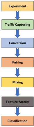
Figure 2: Step 1&2 of detection method construction
2. Related Work
After reviewing the number of research paper, the following comprehensive finding from the literature has been noted down as per below table: - 1. It represents the working approach of various other researcher which is relevant to DNS Tunneling Detection. After analyzing each research paper, it is observed that the accuracy for detecting the DNS Tunneling has been increased subsequently.
Table 1: Description of comparative papers
S.No. |
Year of Publishing |
Approach |
Reference |
Accuracy |
1 |
2018 |
In the research “DNS Tunneling Detection Method Based on Multilabel Support Vector Machine”, a multilabel classification using kernel SVM for the sake of detecting DNS tunneling. |
[17] |
80% |
2 |
2017 |
The authors in this research paper “Comparative Analysis for Detecting DNS Tunneling Using Machine Learning Techniques”, used SVM, NB, and J48 for detecting the malicious DNS packet. |
[11] |
83% |
3. |
2018 |
In the research “DNS Tunneling Detection Using Feedforward Neural Network.” addresses the problem of detecting Domain Name System (DNS) tunneling in a computer network. This paper proposes a machine-learning method of distinguishing tunneling strategies. |
[18] |
83% |
4 |
2020 |
The authors in this research paper “DNS Tunneling: A Deep Learning based Lexicographical Detection Approach” proposes a detection approach based on a Convolutional Neural Network (CNN) with a minimal architecture complexity. |
[10] |
92% |
5 |
2017 |
In this research paper “Detection of DNS tunneling in mobile networks using machine learning”, proposes the use of machine learning techniques in the detection and mitigation of DNS tunneling in mobile networks. Two machine learning techniques, namely One-Class Support Vector Machine (OCSVM) and K-Means have been experimented with. |
[19] |
96% |
6 |
2019 |
The authors in this research paper “A DNS Tunneling Detection Method Based on Deep Learning Models to Prevent Data Exfiltration”, uses a dense neural network (DNN), one-dimensional convolutional neural network (1D-CNN), and recurrent neural network (RNN) on Dataset containing DNS protocols Network packets. |
[12] |
99.90% |
The Table 1 represents the research papers title of related works along with their author and the approach they have used for the detection of DNS Tunneling attack. The accuracy in the table 1 represents how accurate is the machine learning approach of the research in DNS Tunneling attack detection.
From table: -1, we conclude that the method proposed by different authors were different from the method we proposed. Throughout our task we have comprised four different deep learning algorithms together and then individually we compared different features of the algorithms and results into the best among them. While in other research work Machine learning algorithms have been used separately as somewhere support vector machine (SVM) and in another Naïve Bayes (NB) been used. In some papers only two deep learning algorithms been compared [1-D CNN & RNN] and in other paper two machine learning techniques [OCSVM & K-Mean] has been used. Our approach is the unique approach of solving the task and achieved higher accuracy and other features as compared to other research work.
3. Methodology
3.1. DNS Tunneling Tools & Experiment
The Experiment in our paper makes use of the dnscat2 tool to perform DNS Tunneling. dnscat2 being designed to create an encrypted command and control channel over DNS, is used for this paper experiment. The tunneling approach implemented by dnscat2 involves an attacker-controlled system running dnscat2 server software. We used public cloud provider Digital Ocean which provides virtual private servers to install dnscat2 server components. Once active, the dnscat2 server component will listen on User Datagram Protocol (UDP) port 53, presenting an interactive shell to remotely control systems that run dnscat2 client software. dnscat2 client was installed in Kali Linux, launched by specifying the IP or hostname of the server system in the “–host” parameter.
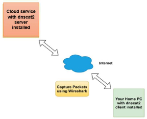
Figure 3: Workflow of DNS Tunneling
Figure 3 shows the workflow of DNS Tunneling attack using the dnscat2 tool. The dnscat client was installed in the targeted user’s system and the dnscat server was installed on the Cloud service provider.
3.2. Dataset
To collect and construct a good quality dataset, a DNS Tunneling attack has been recreated three times and Wireshark has been used to collect a dataset of network packets obtained from the attack. Wireshark is used for capturing and analyzing network packets. While doing the attack three times, Wireshark captured the network packets, and from that three pcap files containing malicious network packets were obtained. Wireshark was also used for obtaining features that contain normal (non-malicious) network packets. Wireshark captures the network packets and the packets can be saved in pcap format. To create a dataset for training and testing purposes, we converted pcap files to CSV files. The Label feature was added to the dataset. The Dataset consisting of DNS tunneled packets was whole labeled as positive along with all the network packets and dataset with normal network traffic packets was whole labeled as negative. Due to unavailability of public data of DNS Tunneling and ethical issue, we found better to create dataset on our own. Table 2 shows the description of the dataset. Table 3 shows the data recorded in each file.
After collecting these files, these have been appended and shuffled the files for training and testing of the dataset and made one dataset. Hence, the total rows formed were 114443 and the total columns formed were 8. Following is a part of the final dataset that has been used in training the model.
Table 2: Features description
Feature |
Description |
Time |
It represents the Timestamp |
Source |
It is the address from where the packets are coming |
Destination |
It is the address where the packets are going to |
Protocol |
It shows the name of the protocol used |
Length |
It shows the length of the captured packet |
Info |
It shows the additional information of the captured network packet |
Label |
This column shows the label 0 or 1 for the row to be malicious or non-malicious |
Table 3: Files description
Files |
Rows |
|
Tunneled Data Files |
First Tunneled Dataset files |
5447 |
Second Tunneled Dataset files |
1444 |
|
Third Tunneled Dataset files |
50331 |
|
Non-Tunneled Data files |
First Non-Tunneled Dataset files |
5447 |
Second Non-Tunneled Dataset files |
1444 |
|
Third Non-Tunneled Dataset files |
50331 |
|
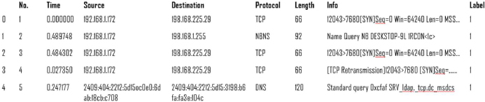
Figure 4: Part of the final dataset used
4. Data Preprocessing
Preprocessing the dataset is always necessary to get more valuable information as there is a famous quote “Garbage in and garbage out”, which means that if we provide the unclean data to any model then in return, we won’t get accurate result from the model. Almost in each & every data related task, Data Preprocessing is performed in order to clean & manipulate the data, conversion of text into binary or numerical values and arrangement of missing values. It plays a crucial role in the field of Machine Learning and Deep Learning domain. In the dataset, Tokenization and padding are involved where conversion of rows from featured dataset into array.
4.1. Network Packets Protocols
The dataset generated consists of a timestamp, related to the network packet generation. The time stamp starts from 0 and measures till the time when Wireshark stopped capturing the packets. The source column and the destination column in the dataset contains the source from where the packet was generated and the destination where the packet was reached. The Protocols obtained were Address Resolution Protocol (ARP), Domain Name System (DNS), Hypertext Transfer Protocol (HTTP), Internet Control Message Protocol (ICMP), ICMPv6, NetBIOS Name Server (NBNS), Secure Shell (SSH), Transmission Control Protocol (TCP), Transport Layer Security (TLSv1.2). For our research, we have considered all the above-mentioned Protocols for the experiment purpose. The length column in the dataset consists of the length of the captured packet. The length of the DNS packet containing DNS tunneling attack detail is observed to be greater than the usual size of the network packet [20]. The info column contains additional information about the network packet.
The generated dataset was exported from Wireshark into csv format. The Wireshark files are saved in pcpa format. The reason behind the export was to ensure the creation of a dataset that can be easily trained over neural networks.
The csv format dataset generated from the pcap file does not contain the label, labeling indicates whether the network query generated was malicious or normal. The label column was added to the column of the csv file. The tunneled dataset was marked with a positive value (1) and the normal dataset was labeled as negative (0).
Mixing algorithm is another step for creating relevant data as input for the machine-learning classifiers. The main requirement for the algorithm is infecting real traffic caps with our tunneling experiments for simulation of the real case when a user performs DNS tunneling in actual traffic. The number of network packets containing tunneled network packets and normal packets are the same. Firstly, all the files generated by three attacks are appended one below the other. Later the labeled dataset was shuffled. This was to ensure that the training, validation, and the testing dataset contains positive as well as negative-labeled network packets.
4.2. Tokenizing and Padding
This step involves the conversion of raw data into those flat features that will be used to train and test the model. Here, the rows of the dataset are converted into an array. Figure 4 shows the array formed from a row.
Now after converting all the rows into their respective format, the total number of arrays obtained and their number of respective labels is 114443. Tokenization involves the splitting of a string into small parts. The reason behind tokenizing is that NLP models cannot be trained with plain text and tokenization is required so that the plain text can be converted to digits. As the tokens are of unequal lengths, padding is required after tokenization. Here padding involves equalizing all the tokens. Vocabulary size having 80000 units, embedding dimensions having 16 units, the maximum length of 120, and padding method was 'post.’
For example, Figure 6 shows the padding of the first sentence. Tokenization of first sentence is as follow: - [2, 2, 34, 33, 35, 32, 3, 4, 5, 6, 7, 23, 30, 36, 8, 11, 14083, 12, 37, 10, 42, 9, 31,7, 24, 26, 25, 27, 28]
Figure 6 is the padded version of the first sentence that has been tokenized. Similarly, all the rows (sentences) are tokenized and padded.

Figure 5: The first row converted to an array
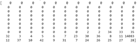
Figure 6: Padding of the first sentence
5. Experiments
5.1. Matrices
A confusion matrix is a technique for summarizing the performance of a classification algorithm. The N x N is created for the purpose of evaluating the performance of the model which is called as Confusion Matrix. This matrix shows the comparison of actual targeted values with predicted values. Among the targeted variable, there are two values named as positive and negative. Here, there are few parameters which plays crucial role in confusion matrix which are True Positive (TP), True Negative (TN), False Positive (FP), False negative (FN).
Table 4: Confusion Matrix format
|
Predicted Values |
|
Actual Values |
Positive |
Negative |
Positive |
True Positive (TP) |
False Negative (FN) |
Negative |
False Positive (FP) |
True Negative (TN) |
False Negative (FN): An instance for which predicted value is negative but actual value is positive.
False Positive (FP): An instance for which predicted value is positive but actual value is negative.
True Negative (TN): An instance for which both predicted and actual values are negative.
True Positive (TP): An instance for which both predicted and actual values are positive.
Precision: Precision indicates out of all positive predictions; how many are actually positive. It is defined as a ratio of correct positive predictions to overall positive predictions. According to formula (1), the precision equals the number of true positives divided by the sum of true positives and false positives.
Recall: Recall indicates out of all actually positive values; how many are predicted positive. It is a ratio of correct positive predictions to the overall number of positive instances in the dataset.
According to formula (2), the recall equals the number of true positives divided by the sum of true positives and false negatives.
F-1 Score: It is harmonic mean of precision and recall.
Mean Square Error: The average of the sum of squares of differences between the predicted and actual values of the continuous target variable.
Here, MSE= Mean square error
n= number of data points
Yi= Observed value
Yi= Predicted value
Accuracy: Accuracy can be defined as the percentage of correct predictions made by our classification model. Despite the widespread usability, accuracy is not the most appropriate performance metric in some situations, especially in the cases where target variable classes in the dataset are unbalanced [21].
Loss: The binary cross entropy loss is actually the only loss we used in our experiment.
Optimizer: Optimizer used was “Adam” for our experiment.
5.2. Implementation
5.2.1. Language and Library
For the implementation purpose, we have used python for programming. The libraries used were NumPy [22], Pandas [23], Matplotlib [24], TensorFlow [25]. NumPy is basically used to deal with array whereas pandas are used to perform data analysis and manipulation operation. Matplotlib is used for visualization and graphical representation in this paper whereas TensorFlow is used for the purpose of creation of deep learning model more efficiently.
5.2.2. Architecture Diagram
Below is the list of Deep Learning Architecture of the training model with a diagrammatic representation of its arranged layers.
The input layer is followed by embedding layer. The batch Input shape is (null, 120). The input shape and length are 8000 and 120, respectively. The output dimension for embedding layer is 16. The input for the Simple RNN layer consisting of 64 units is provided by embedding layer. The activation function for this layer is tanh. Simple RNN layer is followed by flattened layers. The dense layer takes input from the flattened layer. This layer consists of 64 layers with a relu activation function. The next layer is again a dense layer (dense_1) with activation function relu and 6 units. The final layer is a dense layer (dense_2) with 1 unit and a Sigmoid activation function.
The Simple RNN layer of architecture diagram fig(8) is replaced with 1 Dimensional Convolution neural network layer in fig(8). 1-D CNN layer has a linear activation function with 64 filters. It takes the input from embedding layer and has a kernel size of 3.
The Simple RNN layer of architecture diagram fig(10) is replaced with the Bidirectional LSTM layer in fig(10). The Bidirectional LSTM layer has a tanh activation function with 64 filters. It takes the input from the Embedding layer.
5.2.3. Training Model
1-D CNN, Simple RNN, LSTM and GRU algorithms were used for the training purpose. These algorithms were used to train the model over the different split of the dataset. And finally, the model was applied over the testing dataset to check the evaluative accuracy, mean square error, precision, recall, F-1 score, support.
The above Figure11 shows the loss and accuracy over training and validation dataset using the Simple RNN algorithm on 80:20 split. Simple RNN model has been used for training and validation purpose over 80:20 split, the layers used in this model are-Embedded as input layer followed by Simple RNN with 64 units, Flatten, Dense layer with 64 units and Activation function of ‘relu’ followed by Dense layers 6 units with Activation as Relu and Dense layer with 1 unit and activation function of 'sigmoid'. The model was trained for 10 epochs.
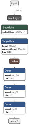
Figure 7: Simple RNN
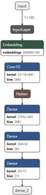
Figure 8: 1-D CNN
The Simple RNN layer of architecture diagram fig(9) is replaced with the Bidirectional LSTM layer in fig(9). The Bidirectional LSTM layer has a tanh activation function with 64 filters. It takes the input from the Embedding layer.
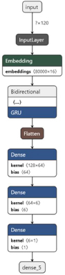
Figure 9: GRU
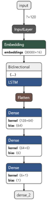
Figure 10: LSTM
Figure12 shows the loss and accuracy over training and validation dataset using the Simple RNN algorithm on 60:40 split. The layers used in this model are-Embedded as input layer followed by Simple RNN with 64 units, Flatten, Dense layer with 64 units and Activation function of Relu followed by Dense layers 6 units with Activation as Relu and Dense layer with 1 unit and activation function of 'sigmoid'. The model was trained for 10 epochs.
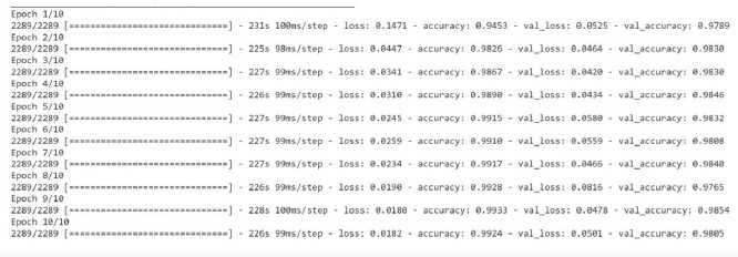
Figure 11: Loss, Accuracy, val. Accuracy & val. loss of Simple RNN model on 80:20 split
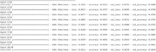
Figure 12: Loss, Accuracy, val. Accuracy & val. loss of Simple RNN model on 60:40 split)
The above Figure13 shows the loss and accuracy over training and validation dataset using the 1-Dimensional CNN algorithm on 60:40 split. 1-D CNN model has been used for training and validation purpose over 60:40 split, the layers used in this model are-Embedded as input layer followed by 1-D CNN with 64 units, Flatten, Dense layer with 64 units and Activation function of ‘relu’ followed by Dense layers 6 units with Activation as ‘’relu’ and Dense layer with 1 unit and activation function of 'sigmoid'. The model was trained for 10 epochs.
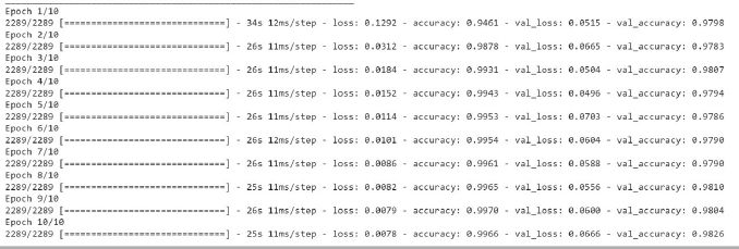
Figure 13: Loss, Accuracy, val. Accuracy & val. loss of 1-D CNN model on 80:20 split

Figure 14: Loss, Accuracy, val. Accuracy & val. loss of 1-D CNN model on 60:40 split
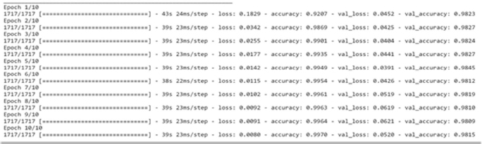
Figure 15: Loss, Accuracy, val. Accuracy & val. loss of GRU model on 60:40 split
The above Figure14 shows the loss and accuracy over training and validation dataset using the 1-D CNN on 60:40 split. GRU model has been used for training and validation purpose over 60:40 split, the layers used in this model are-Embedded as input layer followed by 1-D CNN with 64 units, Flatten, Dense layer with 64 units and Activation function of ‘relu’ followed by Dense layers 6 units with Activation as ‘’relu’ and Dense layer with 1 unit and activation function of 'sigmoid'. The model was trained for 10 epochs.
The above Figure15 shows the loss and accuracy over training and validation dataset using the GRU algorithm on 60:40 split. GRU model has been used for training and validation purpose over 60:40 split, the layers used in this model are-Embedded as input layer followed by GRU with 64 units, Flatten, Dense layer with 64 units and Activation function of ‘relu’ followed by Dense layers 6 units with Activation as ‘’relu’ and Dense layer with 1 unit and activation function of 'sigmoid'. The model was trained for 10 epochs.
Figure 16 gives the idea about LSTM model accuracy for training and validation purpose over 60:40 split, the layers used in this model are Embedded as input layer followed by LSTM with 64 units, Flatten, Dense layer with 64 units and Activation function of ‘relu’ followed by Dense layers 6 units with Activation as ‘relu’ and Dense layer with 1 unit, the activation function of 'sigmoid' and the model was trained for 10 epochs.
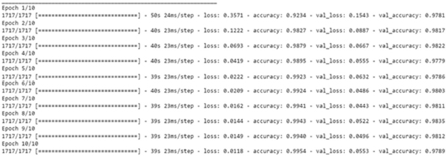
Figure 16: Loss, Accuracy, val. Accuracy & val. loss of LSTM model on 60:40 split
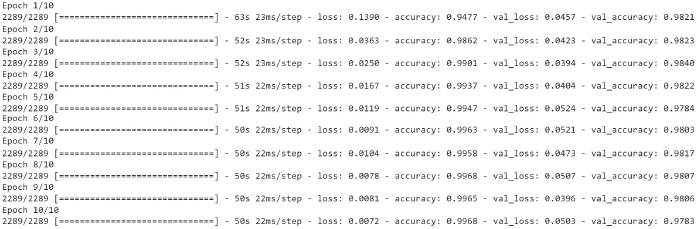
Figure 17: Loss, Accuracy, val. Accuracy & val. loss of GRU model on 80:20 split
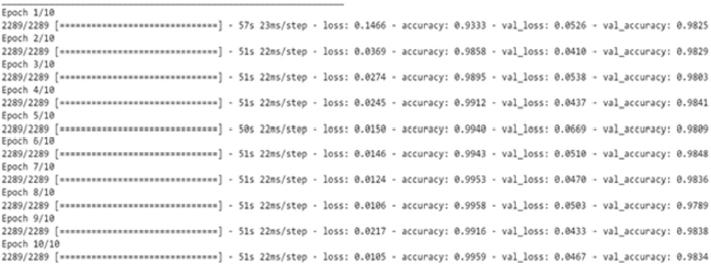
Figure 18: Loss, Accuracy, val. Accuracy & val. loss of LSTM model on 80:20 split
The given Figure17 shows the GRU model training dataset loss & accuracy, validation loss & accuracy 80:20 split. The layers used in this model are-Embedded as input layer followed by GRU with 64 units, Flatten, Dense layer with 64 units and Activation function of ‘relu’ followed by Dense layers 6 units with Activation as ‘relu’ and Dense layer with 1 unit, the activation function of 'sigmoid' and the model was trained for 10 epochs.
The above Figure 18 shows the loss and accuracy over training and validation dataset using the LSTM algorithm on 80:20 split. GRU model has been used for training and validation purpose over 60:40 split, the layers used in this model are Embedded as input layer followed by GRU with 64 units, Flatten, Dense layer with 64 units and Activation function of ‘relu’ followed by Dense layers 6 units with Activation as ‘relu’ and Dense layer with 1 unit and activation function of 'sigmoid' and The model was trained for 10 epochs.
5.3. Results
5.3.1. Accuracy-Loss curve
The Accuracy-Loss curve represents the relation between increasing epoch and loss/accuracy on train/validation data. The X-axis represents the epoch. There are 10 epochs numbered from 0 to 9. The Y-axis represents the accuracy/loss ranging between 0 to 1.
The relation between accuracy/loss and epoch for training data is represented by a blue continuous line. The relation between accuracy/loss and epoch for validation data is represented by a red continuous line.
It is evident from Fig (19) that the training accuracy kept on increasing with the epoch number while the accuracy of validation fluctuates with the epoch number. The training accuracy of 99.24% was obtained on the training data at epoch10 for a simple RNN model over 80:20 split. The training accuracy of 99.24% was obtained on the training data at epoch10f or simple RNN model over 80:20 split. It can be seen in Fig (19) that the training loss kept decreasing with the number of epochs, also the validation loss is decreasing but with fluctuations, with the increasing epochs. While on Testing data, the accuracy of 97.98% was obtained over 80:20 split in a simple RNN model.
It is evident from Fig (20) that the training accuracy kept on increasing with the epoch number while the accuracy of validation fluctuates with the epoch number. It can be seen in Fig (20) that the training loss kept decreasing with the number of epochs, also the validation loss is decreasing but with fluctuations, with the increasing epochs. The training accuracy of 99.20% was obtained on the training data at epoch10 for a simple RNN model over 60:40 split. While on Testing data, the accuracy of 98.22% was obtained over 60:40 split in a simple RNN model.
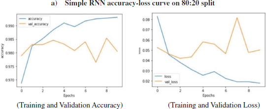
Figure 19: Relation between increasing epoch and loss/accuracy on train/test data
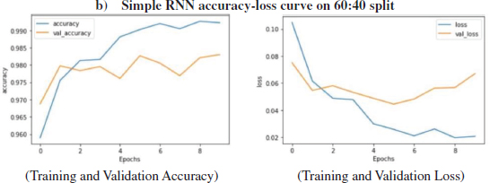
Figure 20: Relation between increasing epoch and loss/accuracy on train/test data
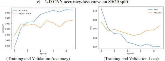
Figure 21: Relation between increasing epoch and loss/accuracy on train/test data
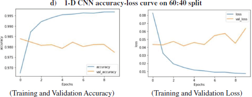
Figure 22: Relation between increasing epoch and loss/accuracy on train/test data
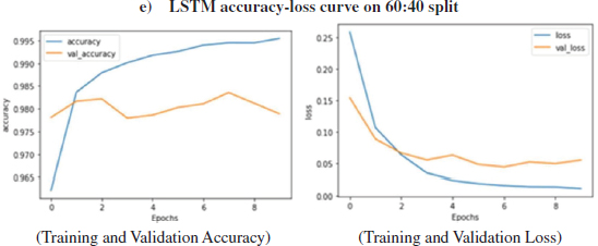
Figure 23: Relation between increasing epoch and loss/accuracy on train/test data
It is clear from Fig (21) that the training accuracy kept on increasing with the epoch number while the accuracy of validation fluctuates with the epoch number. The training accuracy of 99.66% was obtained on the training data at epoch10 for1-D CNN model over 80:20 split. It can be seen in Fig (21) that the training loss kept decreasing with the number of epochs, also the validation loss is decreasing but with fluctuations, with the increasing epochs. While on Testing data, the accuracy of 98.37% was obtained over 80:20 split in 1-D CNN model.
It is evident from Fig (22) that the training accuracy kept on increasing with the epoch number while the accuracy of validation fluctuates with the epoch number. It can be seen in Fig (22) that the training loss kept decreasing with the number of epochs, also the validation loss is decreasing but with fluctuations, with the increasing epochs. The training accuracy of 99.70% was obtained on the training data at epoch 10 for a 1-D CNN model over 60:40 split. While on Testing data, the accuracy of 97.64% was obtained over 60:40 split in 1-D CNN model.
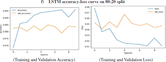
Figure 24: Relation between increasing epoch and loss/accuracy on train/test data
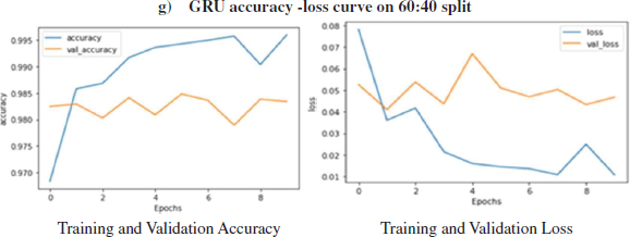
Figure 25: Relation between increasing epoch and loss/accuracy on train/test data
It is evident from Fig.23 that the training accuracy kept on increasing with the epoch number while the accuracy of validation fluctuates with the epoch number. The training accuracy of 99.54% was obtained on the training data at epoch 10 for the LSTM model over 60:40 split. It can be seen in Fig.23 that the training loss kept decreasing with the number of epochs, also the validation loss is decreasing but with fluctuations, with the increasing epochs. While on testing data, the accuracy of 97.73% was obtained over 60:40 split in the LSTM model.
It is evident from Figure: -24 that the training accuracy kept on increasing with the epoch number while the accuracy of validation fluctuates with the epoch number. The training accuracy of 99.59% was obtained on the training data epoch10 for the LSTM model on 80:20 split. It is clear in Fig.24 that the training loss kept decreasing with the number of epochs, also the validation loss is decreasing but with fluctuations with the increasing epochs. While on testing data, the accuracy of 98.42% was obtained over 80:20 split in the LSTM model.
It can be seen in Fig.25 that the training loss kept decreasing with the number of epochs while the validation loss fluctuates with the increasing epochs. It is evident from figure (25) that the train accuracy kept on increasing with the epoch number but the accuracy of validation fluctuates with the epoch number. The training accuracy of 99.70% was obtained on the training data epoch 10 for the GRU model on 60:40 split. While on testing data, the accuracy of 97.86% was obtained over 60:40 split in the GRU model.
It is evident from Figure 26 that the training accuracy kept on increasing with the epoch number, but the accuracy of validation fluctuates with the epoch number. It can be seen in Fig.26 that the training loss kept decreasing with the number of epochs, also the validation loss is decreasing but with fluctuations with the increasing epochs. The training accuracy of 99.68% was obtained on the training data epoch 10 for the GRU model on 80:20 split. While on testing data, the accuracy of 97.90% was obtained over 80:20 split in the GRU model.
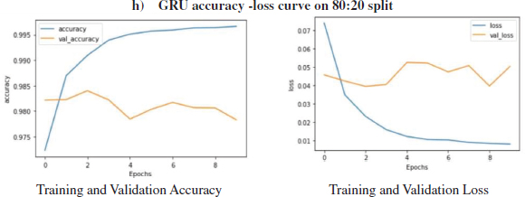
Figure 26: Relation between increasing epoch and loss/accuracy on train/test data
6. Comparative Study
6.1. Algorithm Comparison
The table 5 represent the training accuracy, testing accuracy, validation accuracy, Mean Square error, Precision, Recall, F-1 score of LSTM classifier, GRU classifier, Simple RNN classifier, 1-D CNN classifier over 60:40 & 80:20 training & testing split. The training accuracy, testing accuracy, validation accuracy, Mean Square error, Precision, Recall, F-1 score are represented in percentage i.e., their value lies between 0-100. The next table-6 represents the highest & lowest value of the table-5 metrices.
Table 5: Comparison of Algorithms w.r.t different evaluation measures
Splitting Ratio |
60:40 |
80:20 |
Training Accuracy (%) |
||
1. LSTM |
99.54 |
99.59 |
2. GRU |
99.70 |
99.68 |
3. 1-D CNN |
99.70 |
99.66 |
4. Simple RNN |
99.20 |
99.24 |
Testing Accuracy (%) |
||
1. LSTM |
97.73 |
98.42 |
2. GRU |
97.86 |
97.90 |
3. 1-D CNN |
97.64 |
98.37 |
4. Simple RNN |
98.22 |
97.98 |
Validation Accuracy (%) |
||
1. LSTM |
97.89 |
98.34 |
2. GRU |
98.15 |
97.83 |
3. 1-D CNN |
97.74 |
98.26 |
4. Simple RNN |
98.30 |
98.05 |
Mean Square Error (MSE) (%) |
||
1. LSTM |
2.26 |
1.57 |
2. GRU |
2.13 |
2.09 |
3. 1-D CNN |
2.35 |
1.62 |
4. Simple RNN |
1.77 |
2.01 |
Precision (%) |
||
1. LSTM |
99 |
99 |
2. GRU |
98 |
98 |
3. 1-D CNN |
98 |
98 |
4. Simple RNN |
98 |
98 |
Recall (%) |
||
1. LSTM |
96 |
98 |
2. GRU |
97 |
98 |
3. 1-D CNN |
98 |
98 |
4. Simple RNN |
98 |
98 |
F-1 score (%) |
||
1. LSTM |
97 |
98 |
2. GRU |
97 |
98 |
3. 1-D CNN |
98 |
98 |
4. Simple RNN |
98 |
98 |
6.2. Summary of Comparative Study
From the above table, it can be seen that the lowest training accuracy of 99.20% has been by Simple RNN model over 60:40 split implementation, the lowest validation accuracy is 98.37% by 1-D CNN over 80:20 split implementation and lowest validation accuracy is 98.05 % by Simple RNN over 80:20 split implementation.
Table 6: Summary of Table 4
Features |
Highest (%) |
Lowest (%) |
Training Accuracy |
99.70 (GRU & 1-D CNN over 60:40 split) |
99.20 (simple RNN –60:40) |
Testing Accuracy |
98.40 (LSTM – 80:20) |
98.37 (1-D CNN-80:20) |
Validation Accuracy |
98.34 (LSTM – 80:20) |
98.05 (simple RNN –80:20) |
From the above table, it can be seen that the highest training accuracy of 99.70% has been by GRU model over 60:40 split implementation, the highest validation accuracy is 98.34% by LSTM over 80:20 split implementation and highest validation accuracy is 98.40 % by LSTM over 80:20 split implementation.
6.3. Confusion Matrix
The confusion matrix used in the paper shows the True positive, True negative, False positive and False negative value with different shades of blue, according to their value which ranges from 0 to 1. Extreme blue color indicates a value close to 1. Light blue indicates a value close to 0. The values are rounded off by 2 after the decimal.
6.3.1. Confusion matrix for Simple RNN
From the above figure 27, confusion matrix 22436 (98 %) are True Positive. 421 (2%) are False Positive. 392 (2%) are False Negative. 22529 (98%) are True Negative. The calculated precision Value was {0.98}. The Recall value is 0.98. The f-1 score calculated was 0.98.
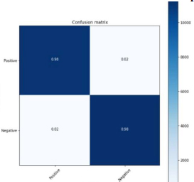
Figure 27: Simple RNN 60:40 split
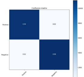
Figure 28: Simple RNN 80:20 split
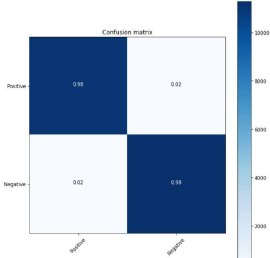
Figure 29: 1-D CNN 60:40 split
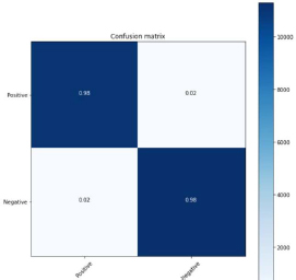
Figure 30: 1-D CNN 80:20 split
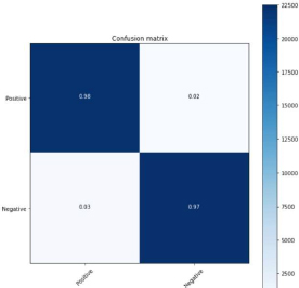
Figure 31: GRU 60:40 split
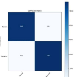
Figure 32: GRU 80:20 split
From the above figure 28, confusion matrix 10970 (98 %) are True Positive. 62 (2%) are False Positive. 400 (2%) are False Negative. 11457 (98%) are True Negative. The calculated precision Value was {0.98}. The Recall value is 0.98. The f-1 score calculated was 0.98.
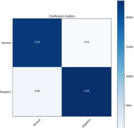
Figure 33: LSTM 60:40 split
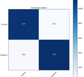
Figure 34: LSTM 80:20 split
6.3.2. Confusion matrix for 1-D CNN
From the above figure 29, confusion matrix 21958 (98 %) are True Positive. 204 (2%) are False Positive. 872 (2%) are False Negative. 22744 (98%) are True Negative. The calculated precision Value was {0.98}. The Recall value is 0.98. The f-1 score calculated was 0.98.
From the above figure 30, confusion matrix 11454 (98 %) are True Positive. 204 (2%) are False Positive. 169 (2%) are False Negative. 11062 (98%) are True Negative. The calculated precision Value was {0.98}. The Recall value is 0.98. The f-1 score calculated was 0.98.
6.3.3. Confusion matrix for GRU
From the above figure 31, confusion matrix 22295 (98 %) are True Positive. 360 (2%) are False Positive. 616 (3%) are False Negative. 22507 (97%) are True Negative. The calculated precision Value was 0.98. The Recall value is 0.97. The f-1 score calculated was 0.975.
From the above figure 32, confusion matrix 11196 (98 %) are True Positive. 204 (2%) are False Positive. 275 (2%) are False Negative. 11214 (98%) are True Negative. The calculated precision Value was 0.98. The Recall value is 0.98. The f-1 score calculated was 0.98.
6.3.4. Confusion matrix for LSTM
From the above figure 33, confusion matrix 21922 (99 %) are True Positive. 138 (1%) are False Positive. 897 (4%) are False Negative. 22821 (96%) are True Negative. The calculated precision Value was 0.99. The Recall value is 0.96. The f-1 score calculated was 0.97.
From the above figure 34, confusion matrix 11134 (99 %) are True Positive. 122 (1%) are False Positive. 238 (2%) are False Negative. 11395 (98%) are True Negative. The calculated precision Value was 0.99. The Recall value is 0.98. The f-1 score calculated was 0.98.
7. Conclusion
This paper has presented a natural language processing-based approach for detecting DNS tunneling. The proposed method has been tested over the generated dataset from the DNS tunneling attack and compared with the performance of different Deep Learning Algorithm. Results showed the LSTM model shows higher accuracy than GRU, 1-D CNN, and Simple RNN model, which implies that the LSTM model tends to identify malicious and non-malicious network packets more often than another mentioned model. The experimental test accuracy showed that the feature extraction method in NLP for detecting DNS tunneling in network packets was found to be 98.42% using LSTM algorithm for 80 :20 split of the generated Dataset. The Precision, recall and f1 score obtain for LSTM algorithm on 80:20 split was 99%, 98% and 98% respectively. Since firewalls and intrusion detection systems detect only specific types of tunneling, this Deep Learning Algorithms can analyze and predict based on previous data provided to it and provide secure networking in the system.
In future, experiment can be performed to Detection of DNS tunneling based on Image Classification Approach. A comparative study of Deep Neural Network (DNN), 2-Dimensional Convolution Neural Network (2-D CNN) and Deep learning Architecture ResNet101 over the generated network packet can prove the best algorithm using for the image classification approach.
8. Conflict of Interest
In this manuscript entitled “Advance Approach for Detection of DNS Tunneling Attack from Network Packets Using Deep Learning Algorithms” has no conflict of interest as declared by the Authors. For this manuscript, no animals or human being has affected. Figure 1,2,3 has been constructed with the tool named as draw.io. No organization has funded for the procedure.
9. References
[1] Sushmita Chakraborty, Praveen Kumar, Bhawna Sinha. “A STUDY ON DDOS ATTACKS, DANGER AND ITS PREVENTION”. 10.1729/Journal.20847.
[2] Roopam, Bandana Sharma. “Review Paper on Prevention of DNS Spoofing”. “International Journal of Engineering and Management Research”. Volume-4, Issue-3, June-2014, ISSN No.: 2250-0758.
[3] Mahmoud Sammour, Burairah Hussin, Mohd Fairuz Iskandar Othman, Mohamed Doheir. “DNS Tunneling: a Review on Features”. “International Journal of Engineering & Technology”. Vol 7, No 3.20 (2018) (Special Issue 20):1-5”.10.14419/ijet.v7i3.20.17266.
[4] Iain M. Cockburn, Rebecca Henderson, Scott Stern. “THE IMPACT OF ARTIFICIAL INTELLIGENCE ON INNOVATION”. “NBER WORKING PAPER SERIES”. http://www.nber.org/papers/w24449.
[5] S Bhatnagar, D Ghosal, M. H. Kolekar, “Classification of Fashion Article Images using Convolutional Neural Networks”, Int. Conf. on Image Information Processing, Jaypee University, Solan, Simla, Dec 2017.1.
[6] D Ghosal, M H Kolekar, “Music Genre Recognition Using Deep Neural Networks and Transfer Learning”, 19th annual International INTERSPEECH Conf, 2018
[7] Ahuja, Dr. Gulshan Kumar, et al. “The Use of Artificial Intelligence based Techniques for Intrusion Detection-A Review.” Artificial Intelligence Review, December 2010, 10.1007/s10462-010-9179-5.
[8] Sabah Alzahrani, Liang Hong. “Detection of Distributed Denial of Service (DDoS) Attacks Using Artificial Intelligence on Cloud”. “2018 IEEE World Congress on Services”. 10.1109/SERVICES.2018.00031.
[9] Kozlenko, Mykola; Tkachuk, Valerii. “Deep Learning based Detection of DNS Spoofing Attack”. Zenodo.10.5281/zenodo.4091017.
[10] Franco Palau, Carlos Catania, Jorge Guerra, Sebastian Garcia, Maria Rigaki. “DNS Tunneling: A Deep Learning based Lexicographical Detection Approach”. Cryptography and Security. arXiv:2006.06122v2.
[11] Mahmoud Sammour, Burairah Hussin, Mohd Fairuz Iskandar Othman. “Comparative Analysis for Detecting DNS Tunneling Using Machine Learning Techniques”. International Journal of Applied Engineering Research”. ISSN 0973-4562 Volume 12, Number 22 (2017) pp. 12762-12766.
[12] Jiacheng Zhang, Li Yang, Shui Yu, Jianfeng Ma. “A DNS Tunneling Detection Method Based on Deep Learning Models to Prevent Data Exfiltration”. “International Conference on Network and System Security”. NSS 2019: Network and System Security pp 520-535. DOI:10.1007/978-3-030-36938-5_32
[13] Willian A. Dimitrov, Galina S. Panayotova. “The Impacts of DNS Protocol Security Weaknesses”. “Journal of Communications, Volume-15, Number-10 October-2020”. doi:10.12720/jcm.15.10.722-728.
[14] Ron Lifinski, Cyber Security Researcher. “How Hackers Use DNS Tunneling to Own Your Network”. https://www.cynet.com/attack-techniques-hands-on/how-hackers-use-dns-tunneling-to-own-your-network/. ISO 27001 & ISO 27032 certified.
[15] Sanjay, Balaji Rajendran, and Pushparaj Shetty. “Domain Name System (DNS) Security: Attacks Identification and Protection Methods”. “International Conference of Security and management (SAM’18)”. ISBN: 1-60132-488-X, CSREA Press.
[16] Kozlenko, Mykola Tkachuk, Valerii Козленко, Микола Іванович. “Deep learning-based detection of DNS spoofing attack”. “Vasyl Stefanyk Precarpathian National University”. 10 December 2019. http://lib.pnu.edu.ua:8080/handle/123456789/8330
[17] Ahmed Almusawi, Haleh Amintoosi. “DNS Tunneling Detection Method Based on Multilabel Support Vector Machine”. Security and Communication Networks 2018(6):1-9. January 2018. DOI: 10.1155/2018/6137098.
[18] Bubnov, Y. 2018. “DNS Tunneling Detection Using Feedforward Neural Network”. European Journal of Engineering and Technology Research (EJERS). 3, 11 (Nov. 2018), 16-19. DOI: https://doi.org/10.24018/ejers.2018.3.11.963.
[19] Van Thuan Do, Paal Engelstad, Boning Feng, Thanh van Do. “Detection of DNS Tunneling in Mobile Networks Using Machine Learning”. Information Science and Applications 2017 Lecture Notes in Electrical Engineering, 2017, p. 221-230. https://doi.org/10.1007/978-981-10-4154-9_26
[20] Greg Farnham. “Detecting DNS Tunneling”. http://www.sans.org/reading-room/whitepapers/dns/detecting-dns-tunneling-34152
[21] UgurTanik GUDEKLI, Bunyamin CIYLAN. “DNS TUNNELING EFFECT ON DNS PACKET SIZES”. “International Journal of Computer Science and Mobile Computing;IJCSMC, Vol. 8, Issue. 1, January 2019, pg.154 – 162”.ISSN 2320–088X.
[22] Travis Oliphant. “NumPy”. https://numpy.org/
[23] Wes McKinney. “Pandas”. https://pandas.pydata.org/
[24] Michael Droettboom, et al, John D. Hunter. “Matplotlib”. https://matplotlib.org/
[25] Google Brain Team. “TensorFlow”. https://www.tensorflow.org/